On the Free Energy Principle
20 July 2020
Created: 2020-07-20
Updated: 2020-12-17
Topics: Biology, Cognitive Science, Physics, Mathematics, Philosophy, History
Confidence: Uncertain
Status: Still in progress
TL;DR - A collection of my thoughts, resources, and related ideas regarding the Free Energy Principle. Discusses Helmholtz machines, causal flow, dynamical systems, markov blankets, thermodynamics, entropy, dynamical systems, variational principles, teleology, philosophy of science, & more.
- Motivation
- Historical Background: The Origins of Teleology?
- Sweeping problems underneath the Markov blanket?
- Introducing the language of Dynamical Systems
- Is there an isomorphism in the inferential engine interpretation?
- Mixing Dynamical Systems + Information Theory
- Philosophy of Science
Motivation
So I stumbled upon this thing called the Free Energy Principle (FEP) back around 2013 when I was looking into how we can distinguish biological living systems from non-living ones. It was a question I was always fascinated by ever since reading books like Schrödinger’s famous What is Life? and Hofstadter’s Gödel, Escher, Bach among many others1 in an attempt to bring meaning to the deluge of chemistry courses I was taking at the time.
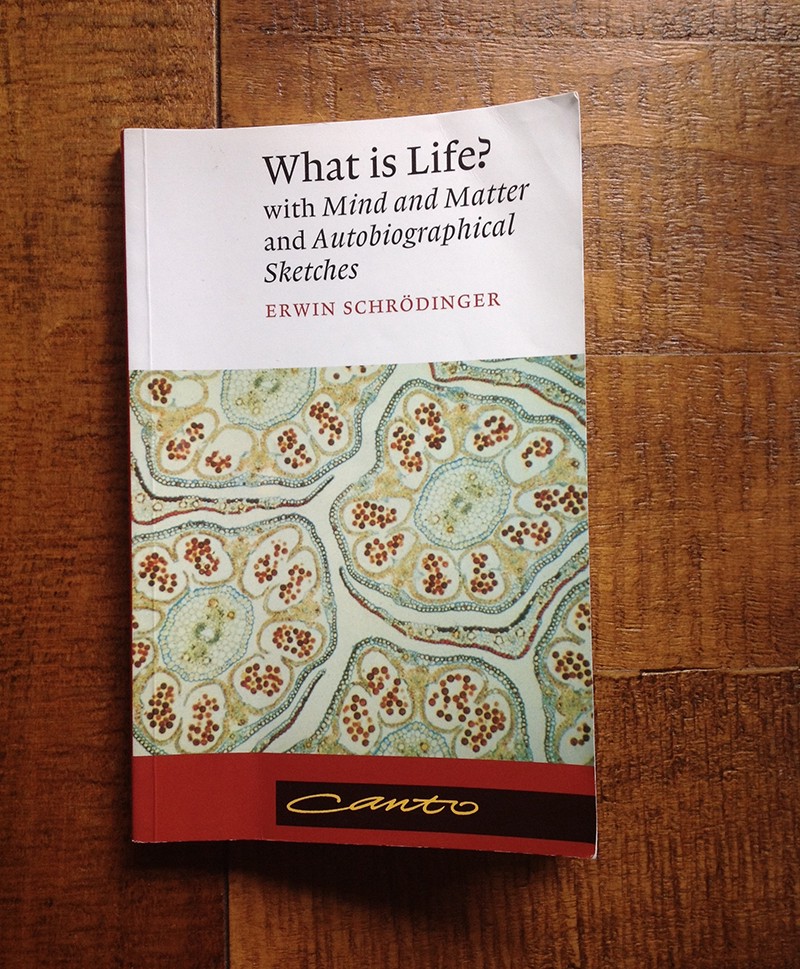 What Is Life? The Physical Aspect of the Living Cell is a 1944 science book written for the lay reader by physicist Erwin Schrödinger. The book was based on a course of public lectures delivered by Schrödinger in February 1943. His lectures focused on one important question: "how can the events in space and time which take place within the spatial boundary of a living organism be accounted for by physics and chemistry?"
Most importantly, I wanted to come up with a way to distinguish living systems from non-living ones in a rigorous, mathematical language. And this mysterious framework kept popping up on my radar when searching through papers. It purportedly was a statement that explained how living systems are special because they can restrict themselves to a limited number of states. Since this resonated well with my own personal theories at the time regarding the key property of life centering around homeostasis and maintaining a particular configuration of molecular arrangements rather than dispersing into the environment, I was immediately hooked.
Over the years I slowly worked my way through the various papers that were pumped out by this person named Karl Friston, who was apparently a superstar in the academic neuroscience world. By coincidence or some self-selection mechanism, I soon began to see his name pop up everywhere. Whether it was during my literature search into this random cognitive robotics professor at UC Irvine whom I previously wanted to work with, or one of my favorite blogs going by the hip name SlateStarCodex2, this Berkeley-based Information & Uncertainty discussion group3 I occasionally joined, this philosopher I really liked4, or even appearing on something as popular as WIRED magazine5, Friston’s FEP just started to show up more and more!
What’s special about the FEP is that it claims that biological systems are able to maintain their structural integrity as a singular system by acting as to minimize their surprise of future events. And the way they did this was by minimizing this term called Free Energy. Friston was claiming that the reason living systems are able to persist through time and thus possess a notion of identity separate from the environment was because they not only inherently modeled the world around them, but they also possessed a fundamental drive to minimize the difference between their internal model of the world and their actual sensory data coming from the external world. And they performed this continuous correction mechanism through both perception and action, either striving to learn more about their world or by actively changing the world to fit within their expectations. Essentially, Friston conceived of biological systems as inference engines.
Now at the time I absolutely fell in love with the FEP. And don’t get me wrong, it still ranks as one of my all-time favorite frameworks of how I perceive the world. But fortunately and unfortunately, as the years progressed I began to specifically seek out criticism against the FEP, and this document serves as a compilation of those associated arguments and my understanding over time. I mainly write this to help clarify my thoughts and consolidate my memories, while also cataloging which resources I was influenced by. Thus, it’s a set of personal notes that are an evolving work-in-progress. With that said, feel free to get in contact if I’ve missed something or made an error somewhere.
Historical Background: The Origins of Teleology?
In tracing the origins of the FEP, a few people like Friston6, Hohwy7, and Andrews8 make the connection between the Free Energy Principle and the Principle of Maximum Entropy by E.T. Jaynes.
The former academics note that Jaynes transformed an originally scientific-materialist, thermodynamic-based set of concepts and associated formalisms and casted them into a more general, probabilistic theory of how we can arrive at some knowledge. This newly created concept was called the principle of maximum entropy and can be considered to be a form of statistical Occam’s Razor. In the original physics-based thermodynamics conception, this acted as a preference for measuring the macroscopic variables of a system like the canonical pressure, temperature, and volume rather than a potentially vast number of underlying microscopic variables such as every particle’s momentum, velocity, and kinetic energy, etc. In the more general, epistemological and probalistic interpretation by Jaynes, it states that we should strive to model the prior data using a probability distribution with the fewest number of assumptions than we have evidence for. It is essentially a claim of epistemic modesty in that the “simplest explanation is usually the right one”. And indeed, this seems to be a principle that many scientists and statistical modelers put to use.3
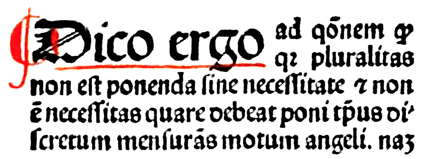 Part of a page from John Duns Scotus's book Commentaria oxoniensia ad IV libros magistri Sententiarus, showing the words: "Pluralitas non est ponenda sine necessitate", i.e., "Plurality is not to be posited without necessity"
It is key to note that the repurposing of this particular mathematical “simplification” apparatus and “minimization” formalism originating in the field of physics has not been isolated to Jaynes alone. In fact, time and time again complex physical systems such as those found in the field of thermodynamics with a vast number of interacting particles have been difficult to model using only classical Newtonian mechanics due to the mathematics getting rather calculation heavy, sometimes even intractably so. One of my favorite philosopher-scientists of all time, German physicist and physician, Hermann von Helmholtz originally conceptualized in his 1881 lecture, On the thermodynamics of chemical processes, something called the thermodynamic potential that measures the useful work obtainable from a closed thermodynamic system at constant temperature and volume, which later became known as Helmholtz free energy (whereas a closely associated Gibbs free energy or free enthalpy is most commonly convenient for systems at constant pressure).
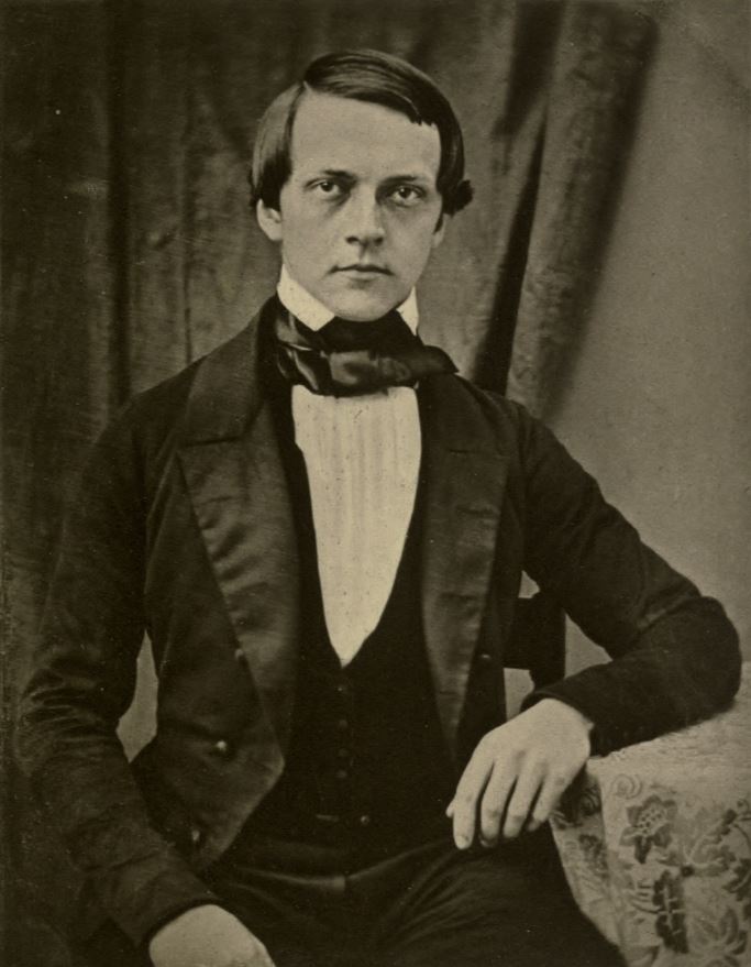 Helmholtz in 1848
To help solve similar problems that Helmholtz faced with physical systems composed of an incredibly complex amount of interactions, alternative reformulations of classical mechanics were developed throughout the history of physics such as that of Lagrangian mechanics that either treated constraints explicitly as extra equations or incorporated them directly via a particular choice of generalized coordinates. Similarly, another alternative reformulation was that of Hamiltonian mechanics which conceptualized something known as the Hamiltonian, which can be said to correspond to the total energy of the system (indeed it is quite useful for describing systems where energy keeps oscillating between kinetic and potential forms, and of which is itself just essentially the Legendre tranform of the former Langragian (function) where the generalized coordinates q_i and time are fixed).
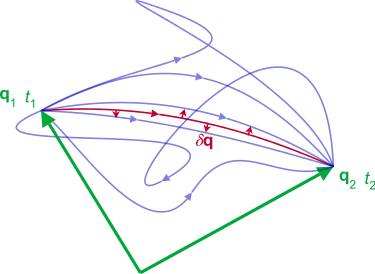 As the system evolves, q traces a path through configuration space (only some are shown). The path taken by the system (red) has a stationary action (δS = 0) under small changes in the configuration of the system (δq).
Similar to the above, physicists such as Feynman were able to use a minimization technique known as a variational method applied to free energy (which originally was physically interpreted as Helmholtz free energy) to solve previous calculation intensive problems. It is important to note that a variational principle in physics is a method for determining the state or dynamics of a physical system by identifying it as an extremum (ie - a minimum, maximum, or saddle point) of a function or functional such as in the case of the previously mentioned time integral of the Lagrangian called the action, which takes a trajectory, path, or history of a system as input and spits out a real number as output. It is key to note the vocabularly of extremums of functions, functionals, paths, etc, which all presuppose a notion that there could be a multitude of possible paths of which one of those could be the optimal path. Indeed talk of multiple variations of paths bakes in a need for a language like the Calculus of Variations which analyzes the variations of a path/functional (ie - by looking at the small changes in a functional’s value due to small changes in the function that is its argument).
 A brachistochrone curve (from Ancient Greek for 'shortest time'), or curve of fastest descent, is the one lying on the plane between a point A and a lower point B, where B is not directly below A, on which a bead slides frictionlessly under the influence of a uniform gravitational field to a given end point in the shortest time. The problem was posed by Johann Bernoulli in 1696. In 1697 he used Fermat's principle of least time to derive the brachistochrone curve by considering the trajectory of a beam of light in a medium where the speed of light increases following a constant vertical acceleration (that of gravity g).
And this is not only isolated to Jaynes, Feynman, or more modern day scientists. Similar principles throughout the history of physics can be found in refraction and optics in the 17th century by Pierre de Fermat (known as his technique of adequality or Fermat’s principle of least time linking ray optics to wave phenomena), Peirre Maupertuis’ 1746 quote “Nature is thrifty in all its actions”, Euler’s 1744 formulation of the action principle, Gauss’ 1829 principle of least constraint, Hertz’s principle of least curvature, Einstein-Hilbert’s 1915 principle of least action, and Noether’s 1915 generalizations connecting underlying symmetries of physical systems with corresponding conservation laws, etc. And this is not only limited to the physical sciences. The overarching appeal to an economy of nature or Principle of Parsimony can likewise be seen all throughout the philosophical world such as in the case of Leibniz’s “best of all possible worlds” where he envisioned God as the great mathematician,
“As is well known, the theory of the maxima and minima of functions was indebted to him [Leibniz] for the greatest progress through the discovery of the method of tangents. Well, he conceives God in the creation of the world like a mathematician who is solving a minimum problem, or rather, in our modern phraseology, a problem in the calculus of variations – the question being to determine among an infinite number of possible worlds, that for which the sum of necessary evil is a minimum.”
Leibniz himself was following a lineage of similar thought generally going under the header of the Principle of Sufficient Reason extending from Anaximander, Parmenides, and Plato, etc, from which Leibniz himself in turn extended this and pollinated fields like mathematics, physics, linguistics, and literature, the latter of which for example can be found in Voltaire’s Candide. In fact, I might be as bold to suspect that much of the philosophical problems surrounding the modern-day attitudes and skepticism of cognitive scientists, biologists, and philosophers regarding the FEP can be traced to the underlying teleogical or “purpose” / “goal-based” character of the action principle dictating Nature picks the optimal course which in turn stem from the philosophical consequences between differential equations of motion and their integral counterparts.
Whereas differential equations are statements about quantities localized to a single point in space or a single moment in time, action principles are not localized to points but rather involve summing over an interval of time or a region of space where it is required that you fix a final state of the system.9 And indeed, similar controversies were brought up against Fermat in 1662(!) because of this principle seemingly ascribing knowledge, purpose, and intent to nature. As we can see, if we accept this historical tracing of lineage of thought, the averse reaction some may have going under the general banner of “A map is not the territory” might be tempered a bit by knowledge that this concept and associated critics have been around for quite some time. Whether or not the teleogical argument is solved seems to depend upon your underlying metaphysical assumptions of the world and potentially your particular philosophical thoughts surrounding the interaction of mathematics and reality.10
 "The miracle of the appropriateness of the language of mathematics for the formulation of the laws of physics is a wonderful gift...[a] striking nature to the miracle that the human mind can string a thousand arguments together without getting itself into contradictions, or to the two miracles of laws of nature and of the human mind's capacity to divine them [shall intersect]"
Sweeping problems underneath the Markov blanket?
To begin investigating how this apparent teleology might crop up, we need to figure out where it is being used and how. First, we need to see how Friston mathematically captures the notion of a system of interacting parts that can be distinguished from its environment. And to do that we need to explain the mathematical object that seems to wrap up all our problems into nice little bundles–the Markov blanket.
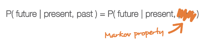
A stochastic or random system / process can be said to exhibit something called the Markov property or memoryless property if its future state depends only upon the state that immediately came before it, not the whole sequence of events that precede it. It reflects the statistical notion known as conditional independence where two events a and b are conditionally independent if and only if the probability of one event a given that the other event b occurred is equal to the probability that a occurred without any knowledge of b having occurred. Basically, the knowledge of event b doesn’t change anything, or in other words, knowing the current state we can’t get any more information about the future by further knowledge of the past. This notion can be represented formally below:
A Markov blanket is essentially a way of statistically demarcating the boundaries of a system of interest separate from its environment. It is a statistical partitioning of a system into internal states and external states, where the blanket itself consists of the states that separate the two.11 We can define a state to be any variable that locates the system at a particular point in state space (which itself is the set of all possible configurations of a system).
In the graphical language of modeling (ie - a Bayesian Network), a Markov blanket represents the set of nodes of all parents of A, children of A, and all the children’s parents other than A. Each node represents an event in time or particular state of the system. Each arrow represents the directed causal influence one node or event has upon another. In Friston’s particular terminology (which deviates a small bit from Judea Pearl’s conception), he further distinguishes the parent nodes of A as sensory states and the children nodes of A as active states, where sensory states are causally influenced by external states and active states are only influenced by internal states.11 Thus, in Friston’s language the existence of a Markov blanket allows us to partition all states into external, sensory, active, and internal states.
 In Probabilistic Reasoning in Intelligent Systems, philosoper and computer scientist Judea Pearl developed computational methods that underlie plausible reasoning under uncertainty based on bayesian belief networks, ultimately creating a theory of causal and counterfactual inference.
Our blanket is labeled Markov because the blanket separates out from the environment both the variables that do not depend on the central node A and the variables that the central node A itself doesn’t depend on. Each variable in the blanket exhibits the aforementioned Markov property, and as such, is all the information we need to know about the system. You might begin to think that we could potentially have nested blankets within blankets, continuing on ad infinitum and you are correct. This is where Pearl further defined an additional term called the Markov boundary which is the minimal or “smallest” such Markov blanket that we could have.
So how do we go about encoding some Markov blanket into the language of mathematics? It is common to encode graphs as mathematical objects called adjacency matrices. An adjacency matrix is a square matrix where each row header and column header represents a specific node and the cross-sectional entries or elements of the matrix indicate whether or not a pair of nodes in that particular row-column pair are adjacent / connected or not. The value of this particular element of the matrix is the probability of one state or node transitioning to the next state or node. This is why we sometimes call this a transition matrix because it represents the transitions from one state to the next.
This adjacency matrix, which we can call A, represents the causal graph of the entire system. From this we can construct a matrix B that represents the Markov blanket only8. Doing some linear algebraic manipulations to get there, Friston defines our new matrix,
\[B = A + A^{T} + A^{T}A\]To further reduce our graph to only those nodes we care about (for instance, our minimal Markov blanket), we can then multiply this matrix B by a binary encoded vector V (a vector of 1s and 0s) representing the nodes we want. If you’ve studied some linear algebra, we can then recall that the eigenvector of a matrix (where a matrix is just a linear transformation / mapping from one space to another) is the vector that maintains its direction under that transformation and only scales to some scalar amount λ. This principal eigenvector can now represent the strength of causal interaction between states, from which we then apply some educated pick of a threshold to group individual states.8
At this point, I think this is where I am maybe not as critical as someone like Andrews where they believe this thresholding to be a post-hoc, intuition-guided, individual researcher-based ascription, and most importantly not “illuminating natural joints”8. In fact, the spectral theory underlying eigendecomposition and thresholding methods is done all the time in vibration analysis (eg - “Can One Hear the Shape of a Drum?”), dimensionality reduction / Principle Component Analysis, Google’s Page Rank algorithm, collaborative prediction, image compression, general clustering problems, and more. I agree that there are many assumptions that go into the mathematics of all of this and indeed it might be wise to keep at the back of our minds the divide between the language we use to describe reality and reality itself, but at the same time I don’t think that this implies that the math itself does not elucidate any insight into the nature of the physical system in question. As mentioned in the previous examples, these representations definitely can provide real-world utility. Whether or not mother nature has latched onto a similar causal mechanism in how biological organisms maintain integrity and govern themselves still seems up for debate.
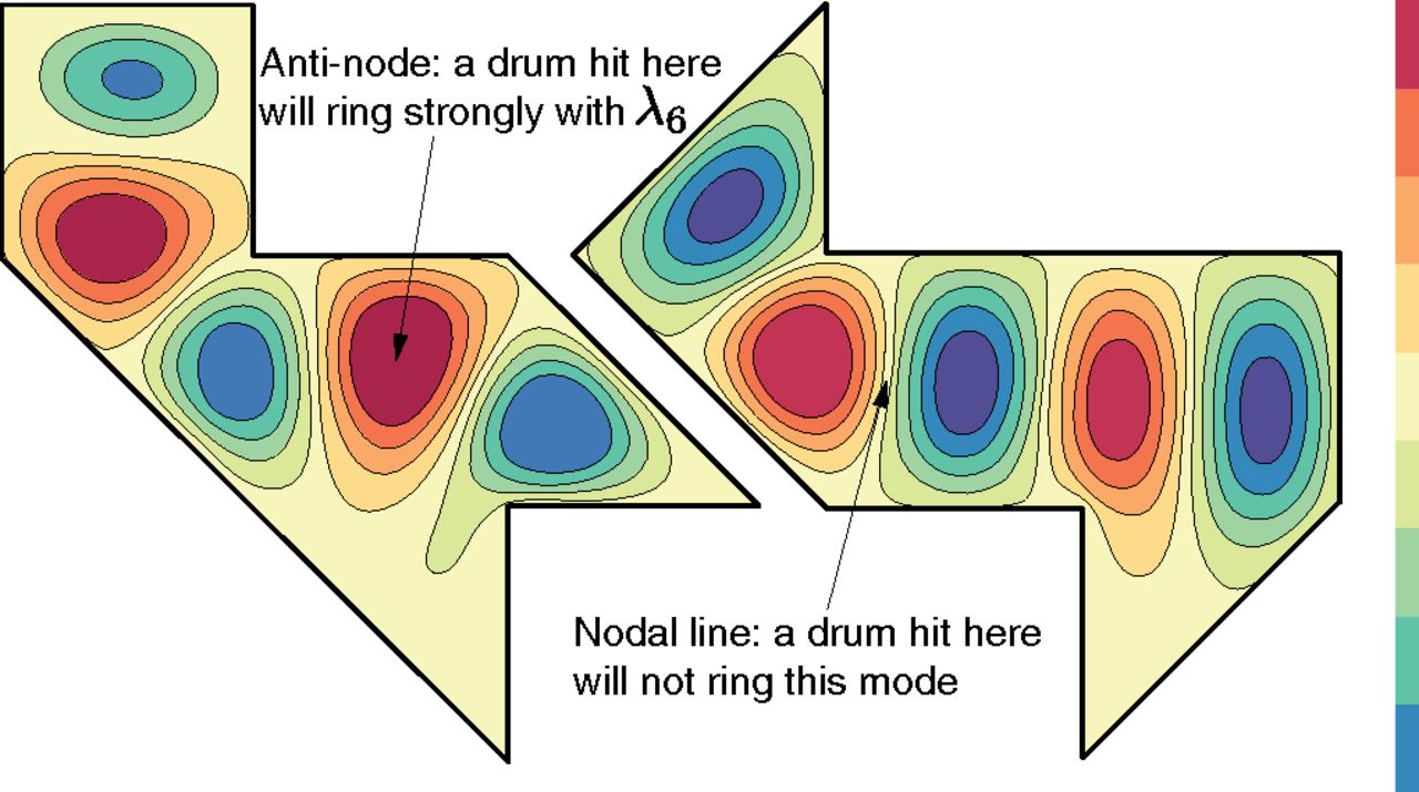 "Can One Hear the Shape of a Drum?" is the title of a 1966 article by Mark Kac in the American Mathematical Monthly. To hear the shape of a drum is to infer information about the shape of the drumhead from the sound it makes, i.e., from the list of overtones. The frequencies at which a drumhead can vibrate depend on its shape. The Helmholtz equation calculates the frequencies if the shape is known. These frequencies are the eigenvalues of the Laplacian in the space. A central question is whether the shape can be predicted if the frequencies are known.
Introducing the language of Dynamical Systems
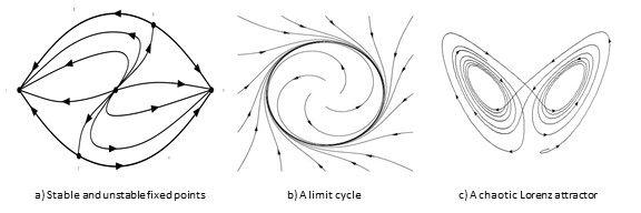
 In the mathematical field of dynamical systems, an attractor is a set of numerical values toward which a system tends to evolve, for a wide variety of starting conditions of the system. System values that get close enough to the attractor values remain close even if slightly disturbed. In finite-dimensional systems, the evolving variable may be represented algebraically as an n-dimensional vector. The attractor is a region in n-dimensional space. In physical systems, the n dimensions may be, for example, two or three positional coordinates for each of one or more physical entities. An attractor can be a point, a finite set of points, a curve, a manifold, or even a complicated set with a fractal structure known as a strange attractor.
Okay, so Friston posits the claim that Markov blankets are pretty much everywhere. From his paper11:
“Here we consider how a collective of Markov blankets can self-assemble into a global system that itself has a Markov blanket; thereby providing an illustration of how autonomous systems can be understood as having layers of nested and self-sustaining boundaries. This allows us to show that: (i) any living system is a Markov blanketed system and (ii) the boundaries of such systems need not be co-extensive with the biophysical boundaries of a living organism. In other words, autonomous systems are hierarchically composed of Markov blankets of Markov blankets—all the way down to individual cells, all the way up to you and me, and all the way out to include elements of the local environment.”
And we can indeed see how our previously defined Markov blanket is a rather broadly-encompassing concept. What isn’t a Markov blanket? I think to help answer that question we need to explore how a system is supposed to maintain its “Markov-blanket-ness”, or in other words, how is a system supposed to keep maintaining its Identity as a distinct set of interacting parts separate from the stuff composing its environment? How does it maintain its integrity without losing its self and dissolving into the environment? How does it keep hold of its Markov blanket?
Friston explains that in order to possess a Markov blanket, a system must minimize something we hinted at before called variational free energy. It is here where someone like Andrews8 comments:
“There is an unfortunate—though understandable—tendency for those first acquainting themselves with the FEP to interpret ‘free energy,’ and other, similarly confounding terminology from the framework, in physical terms. When we speak of heat, energetics, and entropy it can be difficult to shake the feeling that we are talking about some objective, measurable feature of a material system—particle motion, for example…[I] trace the history of the framework in Jaynes, Feynman, Hinton, and Beal because having a handle on this history is necessary in order to grasp the subtle turn away from statistical approximations of physical properties of physical systems to a pure, substrate-neutral method of statistical inference. When we speak of annealing a model in statistical mechanics, ratcheting the temperature of the system up and down in the hopes of bumping it out of local minima, this does not refer to an act of literally injecting energy into a physical system to increase the speed of particle motion. It is a statistical analogue of a physical process. Likewise, the energy and entropy of the FEP are formal analogues of concepts defined in thermodynamics and statistical mechanics with a long history of use in information theory, statistics, and machine learning, in which they have lost their correspondence to any measurable properties of physical systems.”
I can definitely sympathize with this criticism. Adopting mathematics, analogies, metaphors, theories, and jargon from one field to the next doesn’t always transfer over in perfect isomorphic fashion. Some concepts fit. Some stretch. And some break. But just because something breaks or doesn’t perfectly map over from one domain to another doesn’t necessarily mean we should abandon it. Nor should we even jump to the conclusion that something is necessarily broken with the borrowed formalism or apparatus even if it looks like it from the surface (I am not necessarily accusing Andrews of any of these by the way), but maybe rather something doesn’t match upstream in our internal metaphysical beliefs when compared to that of others. Different people might demand different metaphysical conclusions when dealing with reasoning via mathematics and language itself. I mean, I certainly have days where I’m a skeptical scientific Materialist, most days where I’m a hardcore Fictionalist, and yes I admit, even some days where I’m a happy-go-lucky-everything-is-oh-so-beautiful-math Platonist.
Anyway, the reason I question whether or not it really is a metaphysical deathblow that the FEP has lost its correspondence with physical systems is because in the philosophy of physics there are people even questioning our most primitive (and from what I previously thought) well-accepted terms and concepts. Questions such as whether its Force or Energy that is the more real fundamental entity bring up interesting thoughts and consequences12 and in similar sentiment to before can possibly act to temper some of our criticisms.
So getting back to the main topic, what exactly is variational free energy and how is it being minimized? To explain this we need to learn about something called the Fokker-Planck or Kolmogorov Forward Equation. Just as how the velocity of a moving particle is the rate of change of the displacement at some time, the probability density of a continuous real-valued random variable is the rate of change of the cumulative probability at some point. The probability density function is used to specify the probability of the random variable falling within a particular range of values as opposed to taking on any one value (in discrete as opposed to continous cases, this is instead called the Probability Mass Function or PMF). It might be key to note that this probability is given by the area or integral of the variable’s PDF over that range. The Fokker-Planck equation describes how this probability density function of the state of a system changes over time, in essence, how it acts as a trajectory through some abstract space of a system’s set of states.
Our system here is assumed to be under the effect of random perturbations called Brownian motion.13 These random perturbations are assumed to eventually cause the system to undergo an irreversible process known as dissipation in which energy is transformed from some initial form to some final form, where the final form has less capacity to perform mechanical work (ie - although total energy is conserved, not all types of energy are spent equally). So what’s keeping the system from dissipating in its entirety?
 Brownian motion is the random motion of particles suspended in a medium (a liquid or a gas). This is a simulation of the Brownian motion of a big particle (dust particle) that collides with a large set of smaller particles (molecules of a gas) which move with different velocities in different random directions.
Friston conceptualizes the underlying dynamical system as a vector field in three dimensions. Assuming appropriate smoothness and decaying conditions, there’s something called the Helmholtz decomposition, otherwise known as the Fundamental Theorem of Vector Calculus, which states that a rapidly decaying vector field in three dimensions can be broken up into the sum of two components, an irrotational (curl-free) vector field and a solenoidal (divergence-free) vector field.13 This latter solenoidal divergence-free field is shown below:
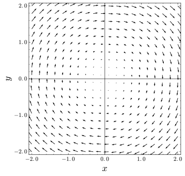 An example of a solenoidal "divergence-free" vector field
Whereas the solenoidal or divergence-free field is known for its property that the field has no sources or sinks (and hence the flow of the solenoidal field can’t diverge), for the purposes of the FEP it is important to note the other former component, the irrotational divergent component.
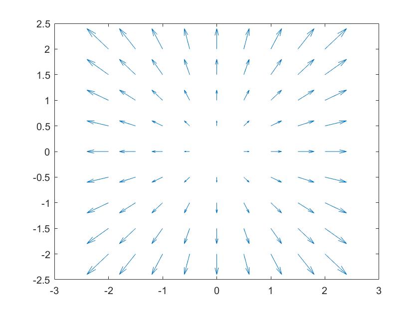 An example of divergence or an "irrotational" component from a source
The other component is called the irrotational vector field or dissipative flow, as shown above. Additionally, when given that the domain is a simply connected open region, the vector field will represent forces of a physical system in which energy is conserved (ie - the reason why they are sometimes called conservative vector fields). For such an irrotational system, the work done in moving along a path in configuration space (the space of all possible positions) depends only on the endpoints of the path, so it is possible to define a potential energy that is independent of the actual path taken (Note to self - Could this be where a portion of the teleology is initially baked-in?)
A really great intuitive explanation of conservative vs. non-conservative vector fields can be given by M.C. Escher’s lithograph print, Ascending and Descending:
 "Ascending and Descending illustrates a non-conservative vector field, impossibly made to appear to be the gradient of the varying height above ground as one moves along the staircase. It is rotational in that one can keep getting higher or keep getting lower while going around in circles. It is non-conservative in that one can return to one's starting point while ascending more than one descends or vice versa. On a real staircase, the height above the ground is a scalar potential field: If one returns to the same place, one goes upward exactly as much as one goes downward. Its gradient would be a conservative vector field and is irrotational. The situation depicted in the painting is impossible."
Friston points out that this dissipative, curl-free flow is the component responsible for counteracting the dissipation caused by the random perturbations of Brownian motion on the underlying vector field (representing the dynamical system).13 This implies that the only remaining probability current is solenoidal, where the term probability current describes the flow of probability in terms of probability per unit time per unit area.
Now this is where things get a bit fuzzy for me. I don’t quite see what is driving the system to be maintained in this state of a rapidly decaying vector field (which is necessary for our condition for the Helmholtz decomposition of the two different vector field components to be allowed).
If I’m understanding Friston correctly, he states that the reason we have this system being maintained in this state is because the non-equilibrium (it is key to note that condition) long-term behavior of any random dynamical system when weakly mixing will after a sufficient amount of time converge to an invariant set of states called a pullback or random global attractor.13
Is there an isomorphism in the inferential engine interpretation?
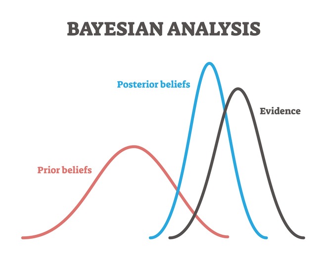 In probability theory and statistics, Bayes' theorem, named after Reverend Thomas Bayes, describes the probability of an event based on prior knowledge of conditions that might be related to the event, and how we can arrive at our new posterior belief given some evidence.
To cast the aforementioned dynamical systems interpretation into the language of probability and information theory we first have to explain how we can capture epistemic notions such as belief and evidence. We also have to formalize a mathematical relationship between how we update our old beliefs with evidence to get new beliefs. We can capture this relationship with the following:
\[\text{New Level of Belief} = \text{Strength of New Evidence} \times \text{Old Level of Belief}\]And then we can put it into Bayesian terms,
\[\text{Posterior Belief} = \frac{\text{Likelihood} \times \text{Prior Belief}} {\text{Marginal Belief}}\]Or more formally…
\[P(H \mid E) = \frac{P(E \mid H) \times P(H)} {P(E)}\]where we let
\[P(H \mid E)\]be read as the “Probability of our Hypothesis being true given that our Evidence is true”. That vertical bar “|” means “given” or “assuming”, which makes the term something called a conditional probability. We can similarly fill in the other terms with this interpretation scheme.
Because the probability of the evidence being true is the same whether the hypothesis is true OR the hypothesis is false, we can then expand out the denominator to get:
\[P(H \mid E) = \frac{P(E \mid H) P(H)} {P(E \mid H) P(H) + P(E \mid \lnot H) P( \lnot H)}\]You can notice that the denominator now contains the sum of all the different types of hypotheses that are compatible with this evidence (in this case we just simplified down to the statement of whether the hypothesis is true or whether it is false). In more complicated cases, we might have many different hypotheses and we’ll have to OR all them together / sum over them all.
It’s also nice to note that we can collapse this equation down to a simple statement that reads that the “probability of some thing H given E is equal to the probability of both H being true AND E occurring, divided by the probability of just E occurring”,
\[P(H \mid E) = \frac{P(E \cap H)} {P(E)}\]where
\[P(H \cap E)\]or written P(H,E) for short, is interpreted as the joint probability of both our Hypothesis being true AND getting this Evidence.
We can recast this into terms of biological systems by thinking of our Hypothesis as what we believe a particular environmental variable currently is, while we can think of Evidence as incoming sensory data. Let’s say we had an organism who cares about a particular environmental variable called temperature, T. And let’s say it receives incoming sensory data S. Then just replacing the variables we can recast Baye’s equation from before into the following14:
\[P(T \mid S) = \frac{P(S \mid T) P(T)} {P(S)}\]We should note that Friston builds his overarching FEP framework based on influence from a colleague of his at the time, Geoffrey Hinton, considered to be one of the founding fathers of the modern Deep Learning paradigm. This framework is based on something called a Helmholtz machine (otherwise known as a Variational Autoencoder when trained via the backpropagation algorithm15). A Helmholtz machine is a statistical engine that can infer the probable causes of sensory input. Every Helmholtz machine is composed of two parts:
1) Bottom-up Recognition Model: This is an internal model of what the organism’s best guess is of the relevant variables that make up its environment. When an organism receives sensory signals it updates this to better reflect and model the surrounding world. This model is formally represented by a probability distribution over all possible values of those environmental variables. Friston calls this probability distribution the “recognition density” or R-density. In our particular example with the environmental variable of concern being temperature, we will denote this R-density as q(T). This is the model that will be updated over time.16
2) Top-down Generative Model: This model reflects an organism’s assumptions about how various environmental variables shape sensory input. It basically reflects how the organism seems to correlate sensory data with environmental states. In our example, this would be interpreted as the organism predicting that if it moves closer to some source of heat, then it’ll receive sensory data signaling that it will get hotter. Like before, this can be formally represented as another probability distribution called a joint density. In Bayesian terms, this is called a joint density because it is calculated as the product of two other densities in turn, the likelihood describing the probability of sensory data given some environmental variable, multiplied by the prior describing the organism’s current belief of the distribution of environmental states. Friston calls this entire joint density or probability distribution the “Generative Model” or G-density. In our example, it can be represented as the joint probability of the environmental variable temperature and its corresponding sensory signal, or P(T,S). This model is what tries to approximate the former bottom-up model, R-density.16
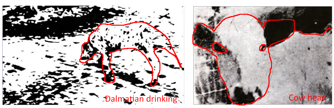 An excellent example from SlateStarCodex that might help prime your intuition: "This demonstrates the degree to which the brain depends on [generated] hypotheses to make sense of [incoming sensory] data. To most people, these two pictures start off looking like incoherent blotches of light and darkness. Once they figure out what they are, the scene becomes obvious and coherent." In other words, once you have a generated a hypothesis, this hypothesis then constrains how you view the sensory data in the future, thus making it difficult to unsee your interpretation when looking at it again. (click image for spoiler)
Because the Helmholtz machine framework envisions organisms as simultaneously receiving sensory data to further model their world in addition to using their internal model of the world to shape how that sensory data is interpreted, we would like some sort of mathematical machinery that would allow us to compare how different our two models or probability distribution are. This machinery is known as the Kullback-Leibler (KL) divergence (aka - relative entropy).
So how do we derive the KL divergence machinery?1718 Let’s say we wanted to compare the posterior probability P(T|S) (what we think the temperature is when given some sensory signal) to our bottom-up recognition model q(T). A simple comparison could be to take the ratio between the two, and indeed this is something called the Likelihood Ratio (LR):
\[LR = \frac{q(T)} {P(T \mid S)}\]Given some set of data composed of a bunch of independent samples, we can take the likelihood ratio for each sample and then multiply them all together like so:
\[LR = \prod \limits_{i=0}^{n} \frac{q(T_i)} {P(T_i \mid S_i)}\]We can then simplify the computation from multiplication to addition by taking the log:
\[\ln LR = \sum_{i=0}^{n} \ln \frac{q(T_i)} {P(T_i \mid S_i)}\]To quickly ground ourselves here, let’s note that if the above spits out values greater than 0 then our q(T) recognition model fits the real-world sensory data better, and if the values are less than 0 then our P(T|S) posterior model fits the real-world sensory data better, and finally if the value is 0 then they fit the data equally well. In summary, the likelihood ratio tells us how many times more probable one model is to another given some data.17
However, let’s say we had a large set of sampled data from q(T). On average, how much would each sample of our q(T) recognition model contribute to better describing the data than our P(T|S) posterior probability model? In essence, we want to calculate the average predictive power each sample from q(T) will bring us when trying to distinguish between q(T) and P(T|S). We can formalize this by sampling N points from q(T) and then normalizing that through division by N.17
\[\ln LR = \frac{1}{N} \sum_{i=0}^{N} \ln \frac{q(T_i)} {P(T_i \mid S_i)}\]Then assuming we do this for an infinite amount of samples from q(T), taking the limit as N -> infinity we then arrive at the expected value,
\[\lim_{N\to\infty} \ln LR = \mathbb{E} \big\{ \ln \frac{q(T_i)} {P(T_i \mid S_i)} \big\}\]Which in the continuous case can be defined as,
\[\mathbb{E} \big\{ \ln \frac{q(T)} {P(T,S)} \big\} = \int_{}^{} q(T) \big\{ \ln \frac{q(T)} {P(T \mid S)} \big\} \,dT\] \[D_{KL}( q(T), P(T \mid S)) ) = \int_{}^{} q(T) \big\{ \ln \frac{q(T)} {P(T \mid S)} \big\} \,dT\]Which gives us our KL divergence equation. And again to ground ourselves, we know that the lower the KL divergence value, the better match we have between our two models. The higher the KL value, the more they are different.17 Although you can think of the KL divergence as a type of “distance” or “measure” between two distributions, it should be noted that the KL divergence is not a true distance given that it is not symmetric and it does not obey the triangle inequality! So just keep that in mind going forward.
To manipulate this into a form where we can begin to distill out some FEP concepts, we can rearrange this using the property of logarithms14,
\[D_{KL}( q(T), P(T \mid S)) ) = \int_{}^{} q(T) \big[ \ln q(T) - \ln P(T \mid S) \big ] \,dT\]Now because we don’t know our true posterior probability P(T|S) since the probability of the temperature given some state is what we are trying to figure out in the first place, we can substitute that term with its equivalent from our Bayesian equation from before.14
\[P(T \mid S) = \frac{P(T,S)} {P(S)}\]Then taking the natural log and using the same property from before we get,
\[\ln P(T \mid S) = \ln \frac{P(T,S)} {P(S)}\] \[\ln P(T \mid S) = \ln P(T,S) - \ln P(S)\]And then subsituting this equation for ln P(T|S) back into our KL divergence equation,
\[D_{KL}( q(T), P(T \mid S) ) = \int_{}^{} q(T) \big[ \ln q(T) - \ln P(T,S) + \ln P(S) \big] \,dT\]We can then do our log property from before in reverse to bring the joint density under as the denominator,
\[D_{KL}( q(T), P(T \mid S) ) = \int_{}^{} q(T) \big[ \ln \frac{q(T)} {P(T,S)} + \ln P(S) \big] \,dT\]And following this up with splitting up the integral,
\[D_{KL}( q(T), P(T \mid S) ) = \int_{}^{} q(T) \ln \frac{q(T)}{P(T,S)} \,dT + \int_{}^{} q(T) \ln P(S) \,dT\]Rearranging the dT terms,
\[D_{KL}( q(T), P(T \mid S) ) = \int_{}^{} q(T) \,dT \ln \frac{q(T)}{P(T,S)} + \int_{}^{} q(T) \,dT \ln P(S)\]Then noting that the total probability of the recognition model sums to 114,
\[D_{KL}( q(T), P(T \mid S) ) = \int_{}^{} q(T) \,dT \ln \frac{q(T)}{P(T,S)} + 1 \times \ln P(S)\]From here we might begin to recognize how we can map our separate terms back to their original high-level concepts. Notice that just like our Helmholtz machine concept required, we are able to now compare our bottom-up recognition model, q(T), with our top-down generative model or joint density, P(T,S). And voilà! This entire term which we can encapsulate as a single variable called F is our one-and-only Free Energy that makes up Friston’s famous theory.14
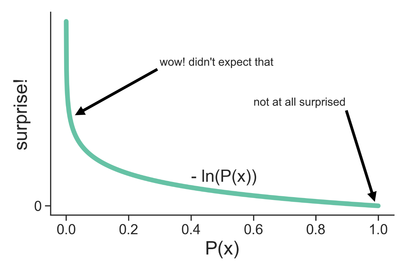
\[F = \int_{}^{} q(T) \,dT \ln \frac{q(T)}{P(T,S)}\] \[D_{KL}( q(T), P(T \mid S) ) = F + \ln P(S)\]We can also notice this separate ln P(S) term at the end. What could that be? Well if we were to visualize the graph of -ln P(S), we’d notice that as the value of P(S) goes up the value of -ln P(S) goes sharply down, and likewise as the value of P(S) decreases the value of -ln P(S) sharply increases.
 See Jared Tumiel's excellent explanation of the mathematics of the FEP. Much of my discussion incorporates his distillation combined with Friston's original papers. Check out the references below for more.
In essence, as the probability of some sensory signal occuring is high, an organism is less likely to become surprised if they do indeed receive that signal. And if the probability of some sensory signal occuring is low but that organism gets a signal anyways, then it’ll sure as heck be surprised to even have received it. As such, we can conceptualize this -ln P(S) term as the Surprise that we received some data.
Further building upon this, Friston noticed that our KL divergence term will always be greater than or equal to zero. Using this we can rearrange the equation so that our Free Energy term lies on the opposing side of our Surprise term.14
\[D_{KL}( q(T), P(T \mid S) ) \geq 0\] \[F + \ln P(S) \geq 0\] \[F \geq -\ln P(S)\]Now we can interpret the above statement that free energy is the maximum amount of surprise an organism can experience upon arriving at some new evidence or sensory data, or more specifically, it is the upper bound on that surprise!
And following the FEP argument by saying an organism acts to minimize their free energy, it is the same thing as saying a biological system acts as to minimize its surprise. In essence, the biological system acts as to create an accurate internal model of the external environment.
We can then tie in the notion of entropy as a measure of how much we expect to be surprised, or our average surprise. A wide, uniform looking distribution where we are more equally unsure of the probabilities of each outcome has more uncertainty and thus on average is more surprising and hence has higher entropy.
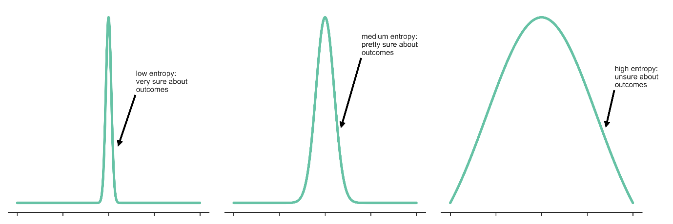
Conversely, a distribution with a very narrow peak would indicate that we know with high probability what our outcomes are, or in other words they lie in a narrow range and so we are more certain and on average less surprised, thus indicating that this distribution would have low entropy. In mathematical simple terms,
\[Entropy = \text{Average Surprise}\] \[Entropy = \mathbb{E} \big\{ Surprise \big\}\] \[Entropy = \mathbb{E} \big\{ -\ln P(S) \big\}\]And so the aforementioned statement about minimization can be distilled down to the statement that a biological system acts as to create an accurate internal model of the external environment, which is the same thing as acting to decrease its (information) entropy!19
Mixing Dynamical Systems + Information Theory
So now that we have a dynamical systems perspective of how a biological system maintains its state and persists throughout some amount of time, and have just shown how a biological system seeks to minimize its free energy, how do we combine these two perspectives?
We can combine these two perspectives by noting something regarding the flow of causal information. Friston notices that we can express the flow of states as a function of their non-equilibrium steady-state (NESS) density. And it is the integrity of this NESS density that is maintained by the irrotational component of the flow under the Helmholtz decomposition. It is important to note this NESS assumption since I think that is the main thing that Friston leverages to identify thing-ness.13 From Andrews8:
“NESS is best understood as the breaking of detailed balance. Detailed balance is a condition in which the temporal evolution of any variable is the same forwards as it is backwards (the system’s dynamics are fully time-reversible). Detailed balance holds only at thermodynamic equilibrium. In nonequilibrium steady state, balance holds in that none of the variables that define the system will undergo change on average over time, but there is entropy production, and there are flows in and out of the system. “
In fact, Friston himself notes that “This is the key result upon which most of this monograph rests”13, mainly that of being able to express the flow in terms of NESS density or surprise. Friston points out from another paper/book20 that the associated NESS density p(x) is the solution to the Fokker-Planck equation, and furthermore that p(x) = exp(P) where P is the scalar potential, which in itself is related to the vector field by way of -∇P, where ∇P is the gradient of P with respect to some Cartesian coordinates x, y, and z. We also just derived above how surprise can be represented by the term -ln p(S).
In other words, the NESS density’s integrity depends upon the irrotatational flow component of the Helmholtz decomposition counteracting the effects of the random perturbations of Brownian motion trying to disperse this NESS density, which implies that we can express the flow into either terms of NESS density or surprise through some basic algebraic manipulations such that our scalar potential P = -ln p(S).13
Philosophy of Science
Is the FEP even a valid scientific principle? Is it even falsifiable? Does it propose any mechanisms? What kind of object is the FEP? Is it better seen as a guiding framework? What are the different types of models?
I think we can start by explicitly describing what we are required to put into the FEP and what we get out.
So in summary, what are all the assumptions we have made with the FEP? I’m trying my best to keep track here, but so far I think we have:
- An appeal to a variational “Occam’s Razor”-like optimization principle
- We can cleanly distinguish discrete, localized causal states that make up our state transition graph/matrix that in turn allow us to represent systems as Markov blankets
- A researcher can come up with the correct thresholds to separate out the specific Markov blanket that we want
- Evidence + Hypotheses are combined in a Bayesian-like algebraic fashion
- Our system is subject to random perturbations or Brownian Motion which causes it to dissipate
- Our system is weakly-mixing which in the long term creates a random attractor
- Our system is at NESS or a Non-Equilibrium Steady State
- There’s a Kullback-Liebler-like measure of divergence between two probability densities of the Recognition Model and a Generative Model
And what do we get out?
- A way to distinguish causal boundaries within a system
- A surprise-like term that can set up an anticipatory framework of interpretation
- An interpretation of two different subsystems within our entire system and the relationship they have between recognizing and generating
- An interconnected formal mathematical framework for parsing our phenomena either in terms of dynamics systems theory or causal inference
Overall, I don’t see anything specific with biology that the FEP spits out, but I do see it potentially carving out a class of models that in turn can provide their biological specifics. We can thus envision the FEP as a type of general framework that specific, higher-granularity biological models might want to slot into and be extended by and constrained by, rather than be a falsifiable model itself. Indeed I think most this seeming concern regarding unfalsifiability8 seems to come baked-in with the assumptions we’ve made, specifically by adopting other general objects that are principles themselves, chief among them being the variational principle and the NESS condition. I single these out because they are the only ones which in my mind have seemingly strong metaphysical consequences associated with each. They each pick out some sort of ideal of which the system moves or strives toward, inherently implying a direction for our causal arrow, of which I can see many academics being wary of since it smells of something like a purpose or goal or essentially a teleology, which does not align with the current and dominant brand of modern-day science.
As such, I think when it comes to the FEP it might be best to maybe adopt an anti-realist or agnostic stance. Maybe instead of the requirement that we demand that the FEP necessarily assert the real existence of anything that might be falsifiable, we can maybe see it in terms providing a useful fiction, thus prioritizing something like utility over Truth in our personal philosophy of science. And more specifically, a utility born with respect to other scientific models that can be gathered underneath its framework (or perhaps even inspired by its framework), rather than singularly providing use by itself.21
 From xkcd, "A webcomic of romance, sarcasm, math, and language"
Resources:
-
The following are books that I read back in undergrad that greatly influenced my thinking with regards to seeking a mathematical framework to capture the definition of living vs non-living systems. These books range from popular science to textbooks. In no particular order, they are: Hoffman’s Life’s Rachet: How Molecular Machines Extract Order from Chaos, Strogatz’s Sync: The Emerging Science of Spontaneous Order, Strogatz’s Nonlinear Dynamics and Chaos, Feldman’s Chaos and Fractals: An Elementary Introduction, Kauffman’s The Origins of Order: Self-Organization and Selection in Evolution, Deacon’s Incomplete Nature: How Mind Emerged from Matter, Mitchell’s Complexity: A Guided Tour, Gribbin’s Deep Simplicity: Bringing Order to Chaos and Complexity, Holland’s Hidden Order: How Adaptation Builds Complexity, and Loewenstein’s Physics in Mind: A Quantum View of the Brain ↩
-
It’s Bayes All The Way Up and God Help Us, Let’s Try To Understand Friston On Free Energy are both blog posts by Scott Alexander from SlateStarCodex. I’d encourage you to read both of these articles to help you gain intuition into the FEP, especially if you are a tad math-averse. They help motivate why we might care about this topic from a neuroscience and psychiatry perspective. Scott is a psychiatrist and famous blogger in the online Rationalist community. ↩
-
The Information & Uncertainty discussion group led by Gerald Friedland at the Berkeley Institute for Data Science (BIDS). These discussions seem to center around the intertwined nature of thermodynamic entropy and information. It was here that I also met Dr. John Harte, another professor at UC Berkeley who is an ecologist doing fascinating work investigating the distribution and abundance of species in ecosystems using a general theory of maximum entropy. ↩ ↩2
-
Surfing Uncertainty: Prediction, Action, and the Embodied Mind is a book by Andy Clark, a philosopher of logic, metaphysics, and cognitive science. In it, he explains the predictive processing framework and how it can be used to explain the role of the mind within the intersection of neuroscience, psychology, and robotics. ↩
-
The Genius Neuroscientist Who Might Hold the Key to True AI by WIRED magazine. This is a special they wrote on Friston and his FEP. ↩
-
A Free Energy Principle for Biological Systems by Friston. From the abstract, “This paper describes a free energy principle that tries to explain the ability of biological systems to resist a natural tendency to disorder. It appeals to circular causality of the sort found in synergetic formulations of self-organization (e.g., the slaving principle) and models of coupled dynamical systems, using nonlinear Fokker Planck equations. Here, circular causality is induced by separating the states of a random dynamical system into external and internal states, where external states are subject to random fluctuations and internal states are not. This reduces the problem to finding some (deterministic) dynamics of the internal states that ensure the system visits a limited number of external states; in other words, the measure of its (random) attracting set, or the Shannon entropy of the external states is small. We motivate a solution using a principle of least action based on variational free energy (from statistical physics) and establish the conditions under which it is formally equivalent to the information bottleneck method.” ↩
-
New directions in predictive processing by Hohwy. ↩
-
The Math is not the Territory: Navigating the Free Energy Principle by Mel Andrews, a PhD student working in the intersection of the philosophy of biology and cognitive science. This document served an incredibly important role as a neutral critic of the FEP for me, and much of my post now incorporates some line of reasoning by them. They not only break down the different components of the FEP, but they briefly go over the history, as well as review the philosophical literature surrounding the area of modeling in general. You can also often find them posting their thoughts on Twitter ↩ ↩2 ↩3 ↩4 ↩5 ↩6 ↩7
-
Apparently, this seems to be eliminated in the quantum mechanical version of the action principle (note to self to expand on this) ↩
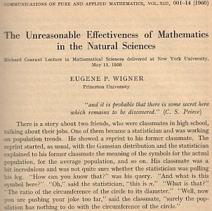
-
The Unreasonable Effectiveness of Mathematics in the Natural Sciences is the title of a famous article published in 1960 by the physicist Eugene Wigner. In it he discusses the seeming miracle of the appropriateness of the language of mathematics for the formulation of the laws of physics. I want to give a quick shoutout to Mihály Bányai, a former PhD student mentor of mine while I was studying at Eötvös Loránd University and working at the Wigner Research Centre for Physics in Budapest, Hungary. I thought the paper was rather simple and boring at the time, but have come to appreciate my mentor’s prescience over the years for urging me to read it. ↩
-
The Markov blankets of life: autonomy, active inference and the free energy principle by Michael Kirchhoff, Thomas Parr, Ensor Palacios, Karl Friston and Julian Kiverstein. From the abstract: “This work addresses the autonomous organization of biological systems. It does so by considering the boundaries of biological systems, from individual cells to Home sapiens, in terms of the presence of Markov blankets under the active inference scheme—a corollary of the free energy principle. A Markov blanket defines the boundaries of a system in a statistical sense. Here we consider how a collective of Markov blankets can self-assemble into a global system that itself has a Markov blanket; thereby providing an illustration of how autonomous systems can be understood as having layers of nested and self-sustaining boundaries. This allows us to show that: (i) any living system is a Markov blanketed system and (ii) the boundaries of such systems need not be co-extensive with the biophysical boundaries of a living organism. In other words, autonomous systems are hierarchically composed of Markov blankets of Markov blankets—all the way down to individual cells, all the way up to you and me, and all the way out to include elements of the local environment.” ↩ ↩2 ↩3
-
Force and energy: which is more real? is post from On Gravity and Levity by Brian Skinner, a professor in theoretical condensed matter physics. In it he discusses the question of whether Force or Energy is more real? He notes that the question “is one to which my answer has changed over the years. The change was a difficult one: force and energy are such profoundly important concepts in physics that to change your view of them is to change your view of all topics that are built upon them (basically, everything). But for me it has been extremely important. Shifting my position from “force is more real” to “energy is more real” was essential for understanding and enjoying advanced topics in physics.” Another somewhat relevant post to the FEP’s inherent teleology is his post on The Universe is a giant energy minimization machine. ↩
-
A free energy principle for a particular physics by Karl Friston. This is probably the most informative write-up on Friston’s theory, but as such it suffers from the fact that it is 148 pages long! From the abstract: “This monograph attempts a theory of every ‘thing’ that can be distinguished from other things in a statistical sense. The ensuing statistical independencies, mediated by Markov blankets, speak to a recursive composition of ensembles (of things) at increasingly higher spatiotemporal scales. This decomposition provides a description of small things; e.g., quantum mechanics - via the Schrodinger equation, ensembles of small things - via statistical mechanics and related fluctuation theorems, through to big things - via classical mechanics. These descriptions are complemented with a Bayesian mechanics for autonomous or active things. Although this work provides a formulation of every thing, its main contribution is to examine the implications of Markov blankets for self-organisation to nonequilibrium steady-state. In brief, we recover an information geometry and accompanying free energy principle that allows one to interpret the internal states of something as representing or making inferences about its external states. The ensuing Bayesian mechanics is compatible with quantum, statistical and classical mechanics and may offer a formal description of lifelike particles.” ↩ ↩2 ↩3 ↩4 ↩5 ↩6 ↩7
-
Friston’s Free Energy Principle Explained An excellent blog post from the more sharper, polymathic, and autodidactic mind of Jared Tumiel. Besides delving into the academic papers, I think this is one of the better alternatives for understanding the mathematics behind the Free Energy Principle. He also has an entire syllabus for understanding the FEP, runs a podcast called Bit of a Tangent and posts his thoughts on Twitter here. ↩ ↩2 ↩3 ↩4 ↩5 ↩6
-
For those adopting the traditional skepticism of whether or not back-propagation can be implemented in biological systems like the brain, see this paper which argues that simple plasticity rules can implement this learning algorithm as efficient as those found in artificial neural networks. The paper addresses the common criticisms and posits several models of biological back-progagation. ↩
-
The free energy principle for action and perception: A mathematical review by Christopher L. Buckley, Chang Sub Kim, Simon McGregor, Anil K. Seth. Besides Friston’s main 148-page monograph which explains and derives each step of his FEP, this is the next best thing towards breaking down the mathematics and their associated concepts. This is also the source that the aforementioned Jared Tumiel seems to draw from. ↩ ↩2
-
Making sense of the Kullback–Leibler (KL) Divergence by Marko Cotra is a really good introduction to the derivation of the Kullback-Liebler Divergence. I modify his derivation to fit our specific terminology with R-density and G-density. ↩ ↩2 ↩3 ↩4
-
Oleg Solopchuk has two really good posts on more applicable process models that use the Free Energy framework. The first being his Tutorial on Active Inference and the second his Intuitions on predictive coding and the free energy principle. Each of them are accompanied by a graphics + a nice derivation of the mathematics. ↩
-
We are noting specifically that this represents Shannon information entropy rather than thermodynamic physical entropy. This is a long running debate in the communities of physicists, computer scientists, and philosophers. I’m making a note here to write a separate post on this issue. ↩
-
Frank, T.D., 2004. Nonlinear Fokker-Planck Equations: Fundamentals and Applications. Springer Series in Synergetics. Springer, Berlin. ↩
-
Indeed, addressing the aforementioned problems is where I think a paper like Andrews shines, drawing from the literature of both Barandiaran and Chemero. They go over the various types of models that exist in the realm of science and explain each with respect to their pros and cons. They essentially explain how the FEP fits into this entire taxonomy. Also tangential note, but Tony Chemero was a former cognitive science professor of mine when I attended Eötvös Loránd University in Budapest, Hungary. My friends Brian Rivera and Mark Wang introduced him to me. Not only did I think he had an incredibly hip hairstyle at the time, but his friendly demeanor even extended to when I randomly bumped into him years later via Twitter and he offered to help me when it came to grad school applications (even after reminding me that I rejected his offer of doing a PhD with him to his face back when I was a cheeky little undergrad 😅). ↩