Organisms as a Special Kind of Information

Created: 2020-11-27
Updated: 2020-01-06
Topics: Biology, Computer Science, Cognitive Science, Physics, Mathematics, Philosophy, History
Confidence: Speculative
Status: Still in progress

TL;DR - Long-form notes recording attempts to model biological organisms using Shannon’s concept of Entropy & Information. This is an effort to disentangle thoughts and see where metaphors + jargon fit, stretch, and break during the mapping.

---

• Motivation
• What is ‘Information’?
• Transmission through Time, not Space
• Predictions
• Resources

---

Motivation

When someone first hears of the concept of applying the notion of ‘information’ and its associated methods to biology, they might come up with a few potential routes of application:

1) Information is manipulated by our brains and so maybe we can analyze how our brains are organizing and transmitting that information. In this particular application we view brains as manipulating information and specific networks of firing patterns as representations of information.

2) Our genetic code stores information about how to build an organism so maybe we can apply information-theoretic tools to analyzing this. In this case we view genes as carriers of information.

3) Organisms communicate with each other all the time through various signals and behaviors and maybe we can mathematically formalize this web of exchanges between them. In this particular application, we view organisms as senders and recipients of information, and language and behaviors as the medium of information.

However reasonable these may seem to us nowadays, over the years many researchers began to borrow methods and concepts that were originally born out of attempts to quantify communication on telegraphs and later the processing done on computers and then re-apply them to the realm of biology on a much more general basis than the above. They began to interpret organisms as information itself.

And this type of thinking is not an isolated incident. Similar ways of thought are echoed throughout the history of science. Such a case can be found following the invention of the mechanical clock where many scientists began to compare the universe itself to a giant mechanical clock. Similar perspectives can be found in people comparing the brain to functioning like a hydraulic pump or even thinking it worked like a steam engine. And one may wonder how much of this historical baggage carried over into our modern day scientists’ preoccupation with finding mechanisms embedded in both a materialist language and philosophy. Likewise, scientists that grew up and were saturated with the successes of the digital computer in our modern age soon began to interpret phenomena through the computational or algorithmic lens metaphor, and viewed the systems found in nature as fundamentally processes of manipulating and transforming information. As the popularly cited Law of Instrument goes, “if all you have is a hammer, everything looks like a nail”.

And while some may laugh at all these metaphors and how quaint and representative they are of their respective times, we should also remind ourselves that it is easy to poke fun of these theories because we possess the gift of hindsight. Maybe instead of ridiculing each of these ways of viewing reality, it might be more productive to view each of these metaphors as not necessarily literally true (they could still be true), but maybe instead currently see them as cases of “make believe” or useful fictions. And then maybe treat these fictions with all the seriousness that we can, seeing just how far we can stretch out their predictive and explanatory value (although there are many more values than just these two when it comes to potentially optimizing our sciences). It’s almost like instead of just simply accepting the map is the territory, we instead mentally sandbox a version of reality and play with that to see how far it leads us.

So treating the aforementioned claim of organisms as information seriously, where can we go from here? I think a good place to start is to address the confusion that has developed over this framework and what we define as ‘Information’. Then I’ll address whether or not there are different kinds of infomation. From there we’ll see if any subset of these can be mapped to the biological realm. In these set of notes I will strive to disentangle some of my own confusions and seek clarification on definitions and claims (it’ll potentially be a long-term work in progress).

What is ‘Information’?

Let’s start with pinning down a definition of Information.

In his famous 1948 paper titled A Mathematical Theory of Communication mathematician Claude Shannon laid out what he thought were the basic elements of communication. It basically took the form of this flow chart:

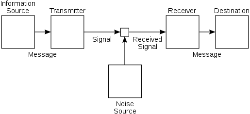Shannon's diagram of a general communications system, showing the process by which a message is sent through a medium or *channel*, potentially being subjected to or corrupted by some noise, and then eventually coming out the other side to be received.

As shown in the image, information was thought of as a set of possible messages sent over a potentially noisy channel and then attempted to be reconstructed by the receiver to have a low probability of error. In his words, “The fundamental problem of communication is that of reproducing at one point, either exactly or approximately, a message selected at another point.”

Because Shannon wanted to know the probability we received one particular message out of all the possible messages we could have received, he captured this notion with the simple statement, p(m) or Pr(M = m). This statement represents the probability that message m is chosen from all possible choices in the message space M.

Shannon then wrapped a negative logarithmic function around it to capture the notion that if we had a 100% probability of receiving a particular message, then we should be completely certain which message we are going to receive. In essence, we already know what would have happened and no information would have been gained by the recipient from the message. In other words, inserting the 100% into our function we get -log(1) = 0 information. The negative is attached to the front because probabilities are given in a range from 0 to 1, and because any fraction in that interval gives a negative number we try to fix that by appending another negative so that they cancel out to make a positive. That way we get to talk about information obtained.

Similarly, Shannon wanted to capture the idea that if we received a compound message consisting of two or more unrelated (mutually independent) messages, then the total amount of information that is transmitted should just be the simple sum of the information obtained individually by each of the messages. Because we usually multiply the probabilities of independent events, logarithms allow us to convert that multiplication into addition, thus capturing the notion of the sum of information.

So what base is this logarithm? The base only affects how much we scale our information and thus represents our units in which we express our information content. By convention we usually go with base 2 so that information is expressed in units of bits (binary digits, 1 or 0). If desired we can also keep this in our usual base 10 decimal digits and use hartleys or go with the natural log and use nats, etc.

So right now we have,

\[Information = - \log{ p(m) }\]

This ‘Information’ is someties called Shannon Information, Self-Information, or Surprisal.

To make this formalism useful, we need to however go a bit farther than this. Shannon further defined a measure of the amount of Uncertainty that a recipient has about which message will be chosen as the average or expected information of a message m from that message space. This uncertainty is called Entropy, Shannon Entropy, or Information Entropy (with the latter especially chosen to distinguish it from Thermodynamic Entropy¹),

\[\text{Uncertainty} = \text{Information Entropy} = H(M) = \text{Average Information}\] \[H(M) = \mathbb{E} \left[ I(M) \right]\] \[H(M) = \sum_{m}^{} p(m) I(M)\] \[H(M) = - \sum_{m}^{} p(m) \log_{2} (p(m))\]

The reason why that p(m) term is inserted in front of the log is because not all messages are equally likely to be received. Some messages might be more probable than others, so we multiply the probability of getting that message times the information from that message, to get the probability of getting that information. What’s nice about this formulation is that if all the messages are equally likely or equiprobable then that p(m) term equals 1/M which makes H(M) = log(M).

It is key to note that despite the mathematical similarities with Boltzmann’s statistical thermodynamic entropy, the two are not necessarily the same thing. While Shannon did borrow the use of the letter H from Boltzmann, Shannon’s informaton entropy is a much more general concept than statistical thermodynamic entropy. Information entropy is present whenever there are unknown quantities that can be described only by a probability distribution. According to E.T. Jaynes, when those probabilities represent particular microstates of a system occuring in order to produce a particular macrostate, then this becomes statistical thermodynamic entropy.

In fact, Jürgen Jost claims¹ that the correct interpretation of H(x) is the average reduction of uncertainty or in other words, the reduction of uncertainty once we learn which concrete value x_i of the random variable X is realized from a known distribution p with probabilities p(x_i).

Jost gives an example¹ where if we have two sides of a coin occurring with equal probability 1/2, then when we flip the coin and observe the outcome we have obtained -log(1/2) = log(2) = 1 bit worth of information (where we use log base 2). Likewise, when we observe the result of a roll of a die, we obtain -log(1/6) = log(6) = 2.58 bits worth of information, etc.

Jost argues¹ that this interpretation is natural and what was intended by Shannon’s axiomatic approach where the properties of continuity, monotonicity, and additivity in his H(x) function were desired. He reminds us that Shannon’s original use for this formalism had to do with sending signals over a phone line. Giving a simplified example¹ of just using Morse code along a telegraph, we get a sender who encodes letters into the Morse code, a line or channel through which the coded signals are transmitted, and finally a receiver who then decodes those signals back into letters. Additionally, we note that our cable line could be subject to external noise, and that our channel capacity is limited since the sender can only send the Morse symbols at some finite speed.

So let’s recast our problem into Shannon’s formalism. We know that the original symbols are composed of the 26 letters of the alphabet plus a stop sign. We also know that each letter is not equiprobable, or in other words each symbol occurs with different relative frequencies in the English text. For instance, the letter e is highly common in English text, occurring 13% of the time, whereas the letter z occurs with a measly 0.074% probability. We will denote this relative frequency for which a particular letter i occurs by its probability p(x_i).

Knowing this, we can then interpret H(x) as the average number of bits transmitted per symbol. From this we can see how to make our encoding to Morse rather efficient. For high probability letters like e we can represent that with a short code, and conversely with lower probability letters like z we can use the longer codes. This minimizes our overall average length of a code word.

However, let’s say that our channel is subject to a lot of noise such that it is difficult to tell apart short codes from each other. Well, to help disambiguate between the short codes, we can make the codes more specific, or in other words, more longer. This increase in information is what Shannon’s formalism allows us to intuitively capture.

Our formalism also allows us to capture the notion of prior knowledge shared between the sender and receiver. We know that concepts like grammar, stylistic choices, personal diction, etc all are used in making us better communicators, and all are used to help constrain our uncertainty. Unfortunately, this is where some conceptual hiccups might take place. In Shannon’s formalism, the information contained in an arbitrary and completely random string of symbols all chosen with equal probability is greater than the information contained from a structured piece of English text! To repeat that, the information obtained is greater in randomness than in order, which might sound counterintuitive. To remedy this conceptual hiccup we have to distinguish the notion of meaning from the notion of information. A meaningful piece of text is not equivalent to a higher amount of information obtained.

I think we can help clarify this by understanding that if a receiver is able to learn something from a structured message, we can grant that they have gotten information. If they were instead given a close to jumbled up message, and were not able to parse it, then they have gotten no information. However, if they were given a jumbled up message, but still were able to parse it, we can say that they have gotten a lot of information. In essence, they reduced their uncertainty the most in the last case, but only reduced their uncertainty by a small amount in the first case.

It is also key to note that the information obtained is not an absolute objective amount of information, but rather relative to what the receiver knows prior to getting the message compared to after reading the message. In other words, Jost notes¹ that the information obtained depends on the prior state of knowledge of the receiver. It is a relative quantity, and in order to formalize that idea we need a concept known as conditional information:

\[p(x_{i}) = \sum_{j}^{} p(x_{i} \mid y_{j}) q(y_{j})\]

where in addition to X we have another random variable Y that can take on a specific value y_j with a probability q_j. The conditional probability p(x_i|y_j) is interpreted as the probability of x_i given that y_j has occurred.

We know from probability that the statement inside that summation above is called the joint probability or the probability that both events ocurr at the same time:

\[p(x_{i}, y_{i}) = p(x_{i} \mid y_{j}) q(y_{j})\]

Knowing this, we can substitute the above inside the summation in the equation prior to that,

\[p(x_{i}) = \sum_{j}^{} p(x_{i}, y_{j})\]

This gives us what is called the marginal probability or the probability p(x_i) occuring regardless of whether or not we know the outcome of the other variable.

Thus, we can define the conditional entropy as the average uncertainty in X given some knowledge of Y. In other words, it is the average amount of information obtained given some knowledge Y. We do this by taking the conditional information -log(p(x_i|y_j)) and multiplying each of those messages by its corresponding probability of occurring p(x_i) (given by our marginal directly above):

\[H(X \mid Y) = - \sum_{j}^{} \sum_{i}^{} p(x_{i}, y_{j}) \log p(x_{i} \mid y_{j})\]

Knowing the above lets us now quantify “the amount of information” (in bits) obtained from one random variable through observing another random variable. We do this through what is called the mutual information between X and Y given by,

\[MI(X : Y) = H(X) - H(X \mid Y) = H(Y) - H(Y \mid X)\]

Where we can substitute for H(X) and H(X|Y) respectively.

Intuitively we can think of the above equation as saying that if we did not know Y at all, our uncertainty comes solely from H(X) (also known as our entropy). However, if we do know Y, then the H(X|Y) term now comes into play and reduces our uncertainty. Anything that is left after this difference is the information that they already shared. In essence, the mutual information is how much knowledge of one of these variables reduces the uncertainty about the other variable, and vice versa. If knowledge of X does not give any knowledge about Y and vice versa, than their mutual information is zero. We should note that no matter what, this mututal information term is alway non-negative, or in other words, if we learn something we cannot increase our uncertainty/entropy, we can only decrease it.

To build upon this further, let’s consider adding another random variable Z. Following the same derivation steps as the above, we can define the conditional mutual infomation as,

\[MI(X : Y \mid Z) = H(X \mid Z) - H(X \mid Y,Z)\]

This statement represents the mutual information between X and Y gained with knowledge Z. We need this Z term to explicitly represent any background knowledge onto which we should condition on, but generally speaking Z can represent any other knowledge like the background context of a situation or even the receiver’s own memory (ie - other facts held in the head).

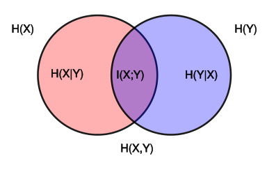Venn diagram showing the area contained by both circles is the joint entropy H(X,Y). The circle on the left (red and violet) is the individual entropy H(X), with the red being the conditional entropy H(X|Y). The circle on the right (blue and violet) is H(Y), with the blue being H(Y|X). The violet is the mutual information I(X;Y).

A somewhat similar looking term MI(X : Y,Z) tells us how much information is gained about X when we know Y and Z together. The theory of information decomposition¹ shows us how Y and Z both individually each on their own and jointly together contribute to this information. It is given by,

\[\text{Mutual Info} = \text{Shared Info} + \text{Unique Y Info} + \text{Unique Z Info} + \text{Complementary/Synergistic Info}\] \[MI(X : Y,Z) = SI(X : Y,Z) + UI(X: Y \ Z) + UI(X: Z \ Y) + CI(X : Y,Z)\]

where SI(X : Y,Z) is the information that both of them have individually (including redundant information is it exists), UI(X: Y\Z) is the information that Y has exclusively, and CI(X : Y,Z) is the information that can only be seen from the combination of Y and Z but from neither of them alone. An example case of the latter synergistic information would be if we took an XOR gate,

y	z	x
0	0	0
0	1	1
1	0	1
1	1	0

where knowledge of both variables y and z determines the third variable x, but knowledge of just y by itself or just z by itself cannot determine x. Neither do they share information either. Thus, the XOR gate only represents synergistic or complementary information.

So let’s summarize really quick what we learned:

1) Information, Shannon Information, or Surprisal

\[I(m) = -log(p(m))\]

2) Entropy, Reduction of Uncertainty, or Average Information

\[H(M) = \mathbb{E} \left[ I(M) \right] = \sum_{m}^{} p(m) I(M) = - \sum_{m}^{} p(m) \log_{2} (p(m))\]

3) Conditional Probability (probability of one event occurring in the presence of a second event)

\[p(x_{i} \mid y_{j})\]

4) Relative Information or Conditional Information

\[p(x_{i}) = \sum_{j}^{} p(x_{i} \mid y_{j}) q(y_{j})\]

5) Joint Probability (probability of two events occurring simultaneously)

\[p(x_{i}, y_{i}) = p(x_{i} \mid y_{j}) q(y_{j})\]

6) Marginal Probability (probability of an event irrespective of the outcome of another variable)

\[p(x_{i}) = \sum_{j}^{} p(x_{i}, y_{i})\]

7) Conditional Entropy (reduction of uncertainly upon given value of another variable)

\[H(X \mid Y) = - \sum_{j}^{} \sum_{i}^{} p(x_{i}, y_{i}) \log p(x_{i} \mid y_{j})\]

8) Mutual Information or Information Gain (measures the information that X and Y share, or how much knowing one of these variables reduces uncertainty about the other)

\[MI(X : Y) = H(X) - H(X \mid Y) = H(Y) - H(Y \mid X)\]

9) Conditional Mutual Information (the mutual information between X and Y gained with knowledge Z)

\[MI(X : Y \mid Z) = H(X \mid Z) - H(X \mid Y,Z)\]

10) Mutual Information with another context variable Z

\[MI(X : Y,Z)\]

11) Mutual Information with Shared Information

\[SI(X : Y,Z)\]

12) Unique Information (solely to that variable)

\[UI(X: Y \ Z) \text{ or } UI(X: Z \ Y)\]

13) Complementary or Synergistic Information (obtained only in the presence of both variables)

\[CI(X : Y,Z)\]

Now that we know what each term corresponds to conceptually and mathematically, let’s see how we can map these to biological concepts…

Transmission through Time, not Space

In Shannon’s application using telegraph wires or cables, he noted that anytime information is transmitted it must go through some channel or medium or carrier process. In this case information is transmitted across space from place A to place B, and the carrier process takes time. In other words, the temporal domain is used.

However, let’s say that instead we want to transmit information not from one point in space to another point in space, but from one point in time to another point in time. To do this we need to inscribe or store the information upon some material carrier in the present to be read again in the future. In other words, the spatial domain is used.

In this latter case¹, the past is the sender, the future is the receiver, and time is the channel. Jost notes that one simple example is some solid structure like a rock. It preserves its information through its structure and transmits that into the future. Or a more abstract example would be how knowledge is passed down from one generation to the next through oral tradition.

In our cases with biological organisms however, we have something more complicated. Instead of a static structural object that we need to transmit through to the future, we have a dynamic set of processes that make up an organism. We have further complications because the structure that we’d like to pass on is the externally expressed phenotype, but the information that actually gets passed on is the internal genotype. Furthermore, an organism also interacts with its environment shaping it such that it makes it more conducive to living and reproduction.

In fact, it could be argued that organisms can reduce the information burden of its genotype in transmitting all the required information by shaping the environment such that it is reproductively favorable and more importantly, stable and predictable. In this way, any organismal structures or phenotypic traits which favor this minimization of information burden on the genotype would be evolutionarily selected for on average. Such traits would be something like enough intelligence to work with one’s hands to create tools, the ability to communicate with others for shared resources and hunting capabilities, etc. Thus, by shaping the environment such that it is less dynamic, more stable, more static, more organized, and more predictable, what organisms are doing is shaping the environmental constraints acting upon them. These new organized environmental constraints then act as a method of offloading this information burden from the encoding organism onto its environment, similar to how a virus offloads its reproductive machinery to the host cells it infects. In other words, if there are potential redundancies that can be found in encoding information, systems will seek to enslave other systems (like that of the environment) to encode that information for them. It’s almost like there is a drive to minimize the burden of encoding information as long as most of the system’s identity remains intact as it transmits itself forward in time.

Anyways, because of the complexities brought about by not only the need to transmit a bunch of nested and mutually-dependent processes instead of static structures, but also the complexities brought about by transmitting processes that dynamically interact with their environment to share information, we need a formalism that can map and be able to assign separate terms to cleanly carve nature at its conceptual joints.

This is where the formalism given above that Jost¹ maps out might prove useful. Our random variable Y can represent the information transmitted through the genome, Z can represent our external contributions, and X can represent the new emerging organism(s). Thus, according the Theory of Information Decomposition given above, our genome Y has a unique information UI that is encoded, shared or redundant information SI between the environment and what is encoded in the genome, and complementary or synergistic information CI between our environmental context Z that the organism dynamically interacts with, which contributes towards the information about our new organism X.

This is where Jost speculates¹ that because any information encoded in the environment does not need to be encoded in the genome, there should be a relatively small amount this. In other words, SI should be small or minimized. Furthermore, because it seems to be rather rare for biological organisms to develop autonomously and completely independent of the environment, our value UI should also contribute little. Thus, the only thing left is for there to be an evolutionary tendency to increase complementary or synergistic information CI as this best makes use of what the environment can provide.

Predictions

A few predictions are thus generated from this framework of maximizing complementary or synergistic information CI (one explicitly mentioned by Jost¹ and others speculated by myself):

1) We cannot evaluate most of the genetic information in isolation from knowledge of the environment from which the organisms develop, live, and reproduce (Jost¹)

2) Systems possess a drive to “couple” with each other in order to each minimize their own shared redundantly encoded information of each other SI, in favor of complementary or synergistic information CI. In other words, systems possess a drive to become individually simpler, but more integrated and mutually complex.

3) Systems that specialize will also be favored. Any system that shares redundant information with another system that it comes in contact with will minimize that redundant information and optimize for processes that help itself and help the other system become more efficient. If two systems start out with slightly different traits that they are more efficient in than the other, they will eventually become specialized in those traits relative to each other.

4) When systems that have a slightly more “general” (perhaps uniform) distribution of traits come into contact with systems that are much more efficient in any particular subset of traits, that more general system is more likely to “enslave” the other slightly more specialized system and offload its information burden to it. This slightly more efficient-in-some-particular-trait-X subsystem will happily join this as it can then offload its information burden in all other traits to the master system except the ones that it is specializing in.

5) The process of coupling systems together with each becoming individually simpler over time means that whenever these systems encounter the circumstance that they are individually separated after a long period of time together, then they will not have the requisite information to survive and perpetuate itself individually and transmit its own information to the future by itself. Thus, interconnectivity breeds robustness at a network level at the cost of being frail at an individual sub-system level.

6) When a system that is less temporally stable (like a living system) and that has a higher burden on maintaining internal memory of its information comes into contact with a system that possesses less of a burden on maintaining memory of its information, the former system will soon offload most of its information to the latter and become simpler at a quicker rate. Relative memory burden / costs might drive the directions of information offload during coupling.

More speculatively,

7) Because information from an organism is offloaded to the environment and eventually is dominated by synergistic information, maybe the claim of multiple realizability and substrate independence is difficult to achieve in practice because it is hard to separate out the “computation” from the “substrate” that it is computed or enacted on, ie - difficult to cleanly separate software from hardware. Maybe the philosophy of functionalism might be false? Maybe to study how living systems come from non-living matter, we can’t simply mathematically model organisms by themselves in isolation, and neither can we just simply pop that organism into a simulated environment and model them both and their interactions, but rather we must mathematically model the organism as being composed of the environment itself (as in the case of cellular automata approaches). Maybe this generative aspect of the environment is key to solving how an environment begins to isolate a part of itself such that that part seemingly is accorded a singular Identity that persists through time and possesses Agency.²

---

Work still in progress…

Personal notes:

1) Add discussion from Pierce’s An Introduction to Information Theory: Symbols, Signals, and Noise regarding the part where information theory melds with physics. Specifically discuss the authors’s construction of a single-molecule variant of Maxwell’s Demon and show how Information could possibly relate to the laws of thermodynamics.

2) Add some examples from Hoffman’s Life’s Rachet: How Molecular Machines Extract Order from Chaos

---

Resources

The gorgeous biological illustration that serves as cover art was done by (in-)famous naturalist and artist Ernst Haeckel.