Generating a Garden with Python

Created: 2020-12-20
Updated: 2020-12-24
Topics: Computer Science, Biology, Cognitive Science, Physics, Mathematics, Philosophy, History
Confidence: Likely
Status: Still in progress

Rewriting Systems Sequence - Part 1

TL;DR - Part 1 of my Rewriting Systems Sequence. A tutorial on experimenting with Lindenmayer systems in Python.

If you haven’t already, check out part 0 of this sequence which gives an introduction to abstract rewriting systems and lindenmayer systems, exploring the philosophical motivation, mathematical theory, practical applications, and major assumptions.

• Rewriting Systems Sequence - Part 1
• Background Review
• Setup
• How to Draw
• Implementing our Production Rules
• Edge vs. Node Rewriting
• Making Tree-like Structures
• Adding Further Realism
• Breaking down the main plotting code
• Moving Forward
• Resources

Background Review

We started off this series wondering if the complex phenomena we see around us could be reduced to just the interaction of simple rules. In general, we were motivated by wondering how living structures build themselves out of non-living structures.

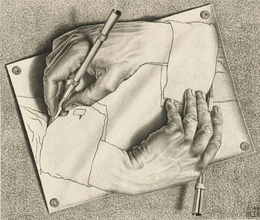Drawing Hands is a lithograph by the Dutch artist M. C. Escher. It is referenced in the book Gödel, Escher, Bach, by Douglas Hofstadter, who calls it an example of a strange loop.

Specifically, we wanted to see if we could model biological systems using a type of formal grammar and parallel rewriting system known as a Lindenmayer system (L-system).

We can recall that an L-system is composed of 4 things:

1) An Alphabet, V, of symbols that can be used to make strings of characters. This alphabet in turn consists of symbols that are of two types: variables, which are symbols that can be replaced, and constants / terminals, which are symbols that cannot be replaced.

2) An initial Axiom string, ω, which is the starting string we begin construction from. It defines the initial state of the system.

3) A collection of Production Rules or Productions, P, that expand each symbol into some larger string of symbols. These rules allow us to recursively generate new symbol sequences.

4) A Mechanism for translating the generated strings into geometric structures. (This is an arbitrary requirement and only used in the case of visualization or other applied purposes)

The rest of this tutorial will now move onto the more practical stuff of setting up your system and converting the aforementioned concepts into Python code.

Setup

If you are a beginner programmer, I’d recommend following the steps below. Alternatively, you can skip these steps and go straight to the code here.

The first thing I’d like to recommend is to set up your programming workflow so that it can handle multiple Python versions, seamlessly transitioning between them depending upon the particular project you are working on at the moment. Not only is this considered good practice in the workplace setting, but it also will prove helpful if we start (inevitably) using different 3rd party packages in our experiments later on in this sequence of posts where these different packages might have dependencies which require conflicting versions of Python.

I’ve ran into these problems multiple times when I’ve least expected it, spent hours troubleshooting and Googling, and during the worst of time-crunches. To save you headaches down the road, we might as well do things the right way from the start.

Now you can probably manually juggle between smartly using your package managers and virtual environments, but why do that when something like Pyenv was built to automatically handle that for you? I recommend following this tutorial to get that set up. I also explain the steps in my code repository, as well as cover any troubleshooting that may arise.

Once you’ve got that done you can install whatever versions of Python you’d like. For this tutorial I arbitrarily chose to go with Python 3.8.0.

How to Draw

From here we need to choose a package that allows us to visualize our output through some graphical plotting method. There are multiple options to choose from like Pycairo, Pillow, Processing.py, Pygame¹, and PyOpenGL, but I chose to go with the humble Turtle package since it follows the “batteries-included philosophy” and comes pre-installed with Python.² I’m next going to go over a few fundamentals you should know about Turtle.

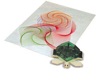Turtle robot toy based on the Logo programming language that aimed to teach children the basics of graphical programming.

After importing Turtle, the first thing you need to do is create a separate window called the screen which acts like your piece of paper onto which you’ll be drawing on. This screen will show your output. You can initialize this screen by the following,

import turtle

screen = Screen()

If you’d like, you can also change the color of the background from the default white to some other color by,

screen.bgcolor("white")

In addition to generating the screen, you’ll need to initialize the turtle object which is shaped like a little arrowhead. This object will act like your pen that does the drawing. In our case, this pen will move in the direction that the turtle is pointing. You can also change the default black color of the turtle’s pen.

turtle = turtle.Turtle()

turtle.pencolor("black")

Finally, you can tell the turtle to move around the screen with the .forward() and .backward() commands, with the given number being the amount of units it will move in that direction. Similarly, you can tell the turtle to change direction with the .left() and .right() commands by giving it a number that specifies the degrees of the angle. For instance, let’s say I wanted to draw a box,

turtle.forward(100)
turtle.right(90)
turtle.forward(100)
turtle.right(90)
turtle.forward(100)
turtle.right(90)
turtle.forward(100)

screen.exitonclick() 

Where that last command screen.exitonclick() allows the window to stay open until we click on it, rather than normally disappearing after the drawing is done. This will let you see your picture after it is done.

Turtle drawing a square.

A few other useful commands such as lifting the pen up/down, going back to the origin, and changing the thickness of the pen are as follows,

turtle.penup()
turtle.pendown()

turtle.home()

turtle.pensize(5)

Other than that, I’d encourage you to check out this Turtle tutorial here if you’d like to know more.

Implementing our Production Rules

Now that we know the basics of how to draw with Turtle, let’s figure out how we can map our aforementioned L-system concept of Production Rules to our Turtle drawings. This is what we mean by having a Mechanism that generates geometric objects from our original data structure of strings. This is also where much of Prusinkiewicz’s contribution was made to the work of the original textbook, The Algorithmic Beauty of Plants.³

We can define the state of the turtle using the triplet (x, y, α), where the first two arguments are the Cartesian coordinates representing the turtle’s position in our window, and the third argument is the angle or heading representing the direction the turtle is facing. Given some step size d and angle increment δ, we can represent the turtle’s path as a string of symbols using the following 4 character mappings⁴:

F: Move forward a step length d. This allows us to change the former state of the turtle to the new state (x’, y’, α), where x’ = x + dcos(α) and y’ = y + dsin(α). A line segment between points (x, y) and (x’, y’) will be drawn. This is our turtle.foward() command.

f: Move forward a step of length d without drawing a line. This is our turtle.penup() command.

+: Turn left by angle δ. The next state of the turtle will now be (x, y, α+δ). The positive orientation of angles will be counterclockwise. This is our turtle.left() command.

-: Turn right by angle δ. The next state of the turtle will now be (x, y, α − δ). This is our turtle.right() command.

What’s neat about this mapping is that we can now interpret a specific state of the system as string composed of some combination of these 4 symbols.

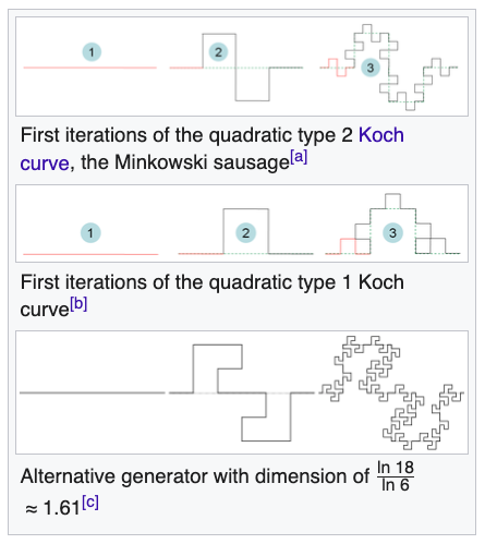
To help build intuition, let’s do a concrete example of an L-system called the Minkowski Sausage (named because of its casual resemblance to sausage links) arranged into a four sided polygon (ie - a square) which in turn is called a Minkowski Island (because it loops back to eventually form an enclosed region).

Our initial state or Axiom ω is given by the string:

ω : F − F − F − F

Which means our initial string tells us to go Forward, Right, Forward, Right, Forward, Right, Forward. In other words, our initial state tells us that we’ll be drawing a box.

And our Production Rule p that explains how we rewrite our given current state to output the next state is given by the rule:

p : F → F − F + F + F F − F − F + F

Which means every symbol that represents Forward is replaced by the following string of characters given after the arrow.

Now if we let our iterations n = 0, this means that no production rules will be applied and we’ll stick with our original Axiom string ω that specifies a box. In our geometric terms this is called the initiator.

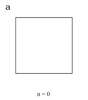Final Turtle drawing of a n=0 Minkowski Island.

However, if let our Axiom undergo one iteration or apply the production rule / rewriting once to get a new string, we’ll have to set our n = 1 (in our geometric terms, this new successor sequence is called our generator) and we get the following,

Turtle drawing an n=1 Minkowski Island.

Likewise, if we apply our production / rewriting rules twice for n = 2, where we feed each previous output string into the next iteration we get the following,

Turtle drawing an n=2 Minkowski Island.

And bumping it up to n = 3 we get,

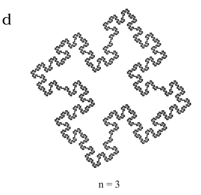Final Turtle drawing of an n=3 Minkowski Island.

…etc.

As you can see, this Mechanism for translating strings to geometric objects can be specified in a rather simple way to generate seemingly complex objects. And we did all this with a single production rule in our examples!

How each part of the Minkowski sausage is just a smaller version of the previous stage.

Using the same starting Axiom ω and just switching up our production rules, Prusinkiewicz and Lindenmayer show how we can generate a startling amount of beautiful structures⁴,

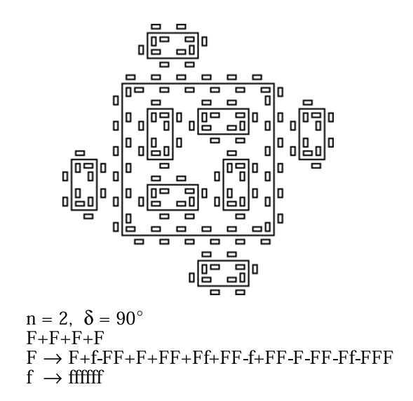From *The Algorithmic Beauty of Plants* pg. 9

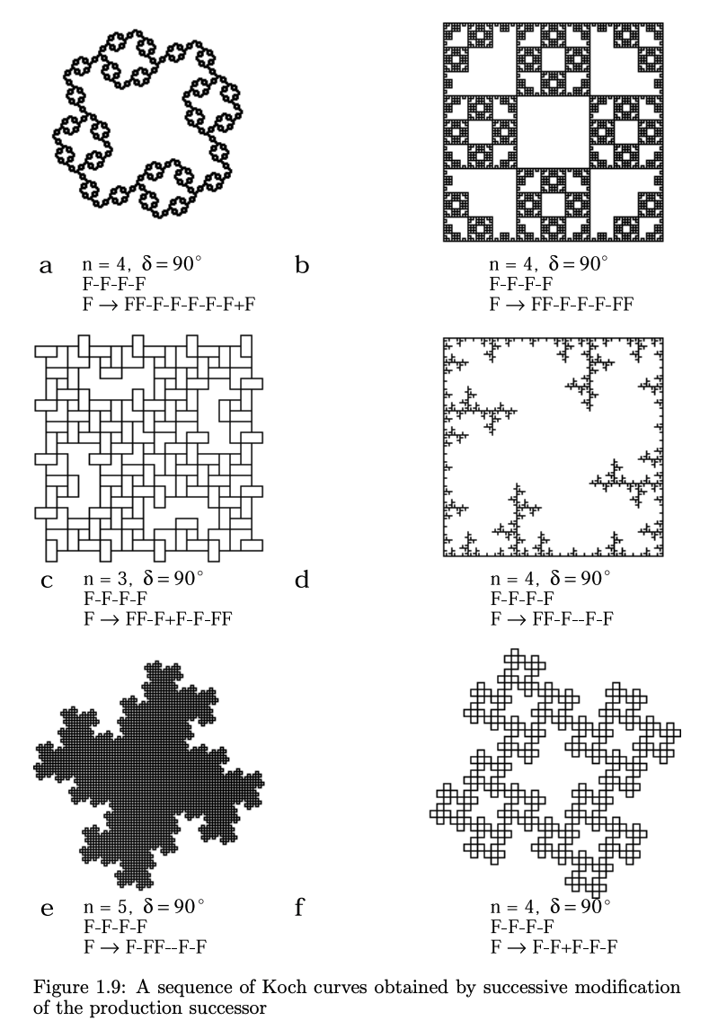From *The Algorithmic Beauty of Plants* pg. 10

From *The Algorithmic Beauty of Plants* pg. 11

Edge vs. Node Rewriting

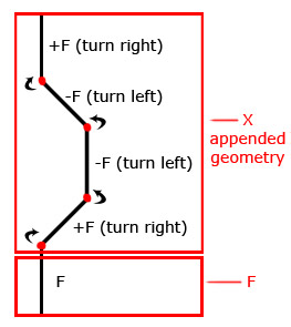
So now that we know how rewriting systems replace some character, substring, or set of symbols with another string of symbols, what if we wanted to append that new string instead? This is where Prusinkiewicz and Lindenmayer explain that there are two types of rewriting mechanisms. The first type is called Edge Rewriting and is what we did before with replacing symbol(s) with other symbols. The second type is called Node Rewriting and occurs when we append new symbol(s) instead. We can specify the latter formally by using a variable such as X like in the following example⁵,

L-System: Simple Example of Node Rewriting

Axiom: FX

Rule: X = +F-F-F+FX

Angle: 45

All that variable X does is act like a logical place-holder for symbols that do matter like F, +, and -. In other words, it is logically relevant to the L-system, but not graphically or physically relevant. Our Turtle program does not move nor draw anything when it sees it. In summary, that variable X does not have a graphical interpretation and does not show up in our final image,

From the personal research of Selcuk Ergen.

There are many interesting things to note about Node Rewriting⁶, but the biologically relevant property of this rewriting scheme is that it allows us to fill a given region by a self-avoiding curve. This self-avoiding property is important if we don’t want our trees to intersect at later points or overlap (for example, it would be like a leaf growing into another leaf and then maybe a new branch coming off of that merger).

Self-avoiding walks on a square lattice by Nathan Clisby. This is from a paper discussing its connection to physics topics like spin systems and renormalization.

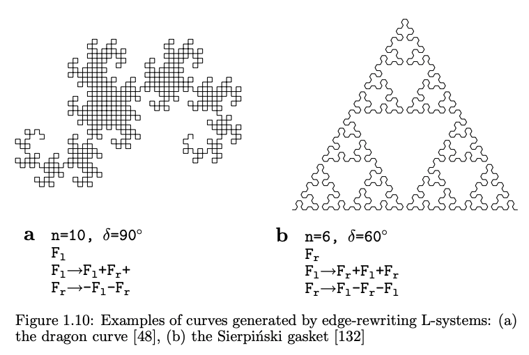
With that said, you can choose to interpret your system by either using an Edge rewriting scheme, or Node rewriting scheme, or both. Neither approach is general, nor are they disjoint from each other.⁴

Self-avoiding walks can also be popularly seen in the classic 1970s game of Snake where a player maneuvers a line which grows in length and has to avoid crashing into itself.

Making Tree-like Structures

So far, our geometric mapping mechanism allows us to interpret a character string as a sequence of individual line segments denoted by F, alternating the direction with + and - respectively. Ultimately, this mapping will only allow us to topologically sketch out a single line. To be able to model something more complex like the tree-like branching (aka - dendritic or arboreal) nature of plants, we’ll need a way to add a little more graph-theoretic structure to our mapping mechanism.

We can do this by specifying the splitting up of a line segment from a root or base into one or more edges that we’ll call branch segments. We’ll call a line segment followed by one or more line segments an internode, and a terminal line segment an apex.⁴

The lateral bud is found at the node on a stem allowing sideways growth. The apical bud (sometimes called the terminal bud) is the top bud at the main growing point of the plant.

If our tree possesses a direction (like in our real world where plants grow upwards and outwards from a common base), then we’ll specify that our edges have to be labeled and directed, and we can call this tree a rooted tree.⁴

We can further create a specific kind of rooted tree called an axial tree. An axial tree is a tree where at each of its nodes there is at most one outgoing straight segment that we’ll be keeping track of separate from the rest. All other remaining edges will be called lateral or side segments⁴, similar to how there is usually one main branch of a plant growing upward, with one or more lateral growths coming off of that main branch on the peripheries.

So what exactly is an axis for a plant? We define an axis as a sequence of line segments in which the following conditions hold:

1) The first segment in the sequence originates at the root of the tree or as a lateral segment at some node. In other words, we want to know that the axis is some branch that has a starting point that it branches from, whether that’s on the ground or at some budding point.

2) Each later / subsequent segment is a straight segment. Basically we want to know that it continues in some straight line.

3) The last segment is not followed by any straight segment in the tree.

So basically what all this means is that an axis is what we call a branch or like a mini-tree that is itself an axial sub-tree.⁴ This “axial-ness” is our self-similarity property showing up and is what will allow us to define statements recursively.

To keep track of our axes / branches, we’ll need to order them. We call the axis orginating at the root of the entire plant as having order zero. In general, the axis coming off of a lateral segment of an n-order parent axis has an order n+1. The following diagram⁴ might help show you what’s labeled what,

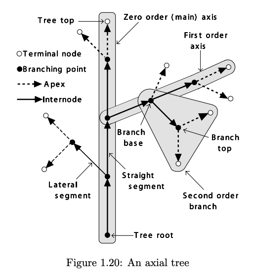From pg. 22 of *The Algorithmic Beauty of Plants*.

And a sample tree illustrating this axis property in action⁴,

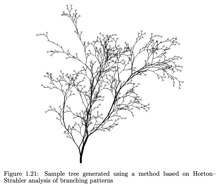From pg. 22 of *The Algorithmic Beauty of Plants*.

So how do we represent this branching structure programmatically in our Turtle notation? Since our underlying data structure is a string of symbols, all we have to do is add 2 more symbols, the open bracket [ and the closed bracket ]. This is why these deterministic & context-free L-systems are sometimes called Bracketed OL-systems.

New symbols⁴:

[: Push the current state of the turtle onto a pushdown stack. The information saved on this stack contains the turtle’s position and orientation (and potentially other information like color or width of the lines). It functions like an input into our storage mechanism.

]: Pop the state from the stack and make it the current state of the turtle. No line is drawn. In general, the position of the turtle might change. It functions like an output from our storage mechanism.

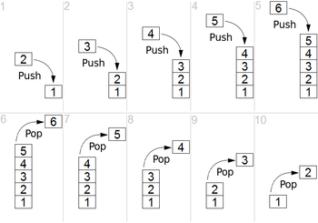Simple representation of a stack runtime with push and pop operations.

Thus, in essence, these brackets are acting as a type of memory or storage mechanism for our strings. And if you recall, each string is a state. So this memory mechanism is a variable that basically records states of our system.

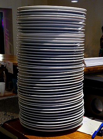Similar to a stack of plates, adding or removing is only possible at the top. In our metaphor, each plate represents a substring of symbol(s) composed of F, f, +, -, etc.

Below are a few examples of what these new bracket symbols allow us to do,

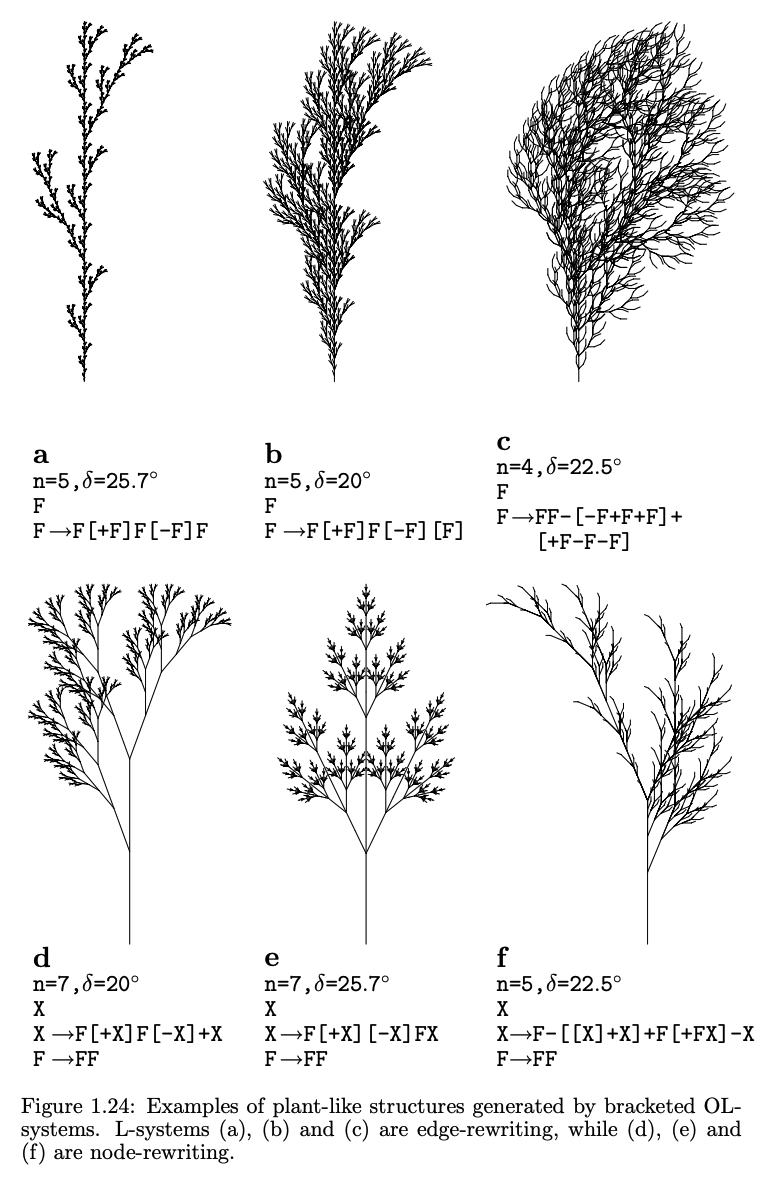From pg. 25 of *The Algorithmic Beauty of Plants*.

And adding in new variables like color and leaves, and modifying our tree-structure to incorporate 3-dimensions we can get something like the following,

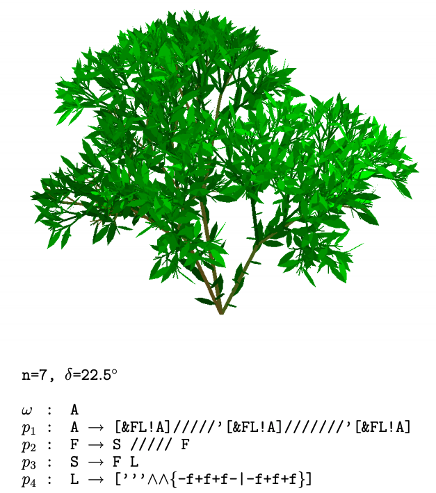Showing a 3-dimensional bush-like plant from pg. 26 of *The Algorithmic Beauty of Plants. The &, ∧, \, /, and | symbols handle the newly added 3D directions. The ! symbol decrements the diameter of segments. The ` symbol increments the current index of the color table for the leaves. And the { and } handle the boundaries of the leaves.

Adding Further Realism

In all the examples we have shown so far, we have dealt with production rules that are deterministic. That is, they always occur whenever it is possible that we can apply them. Unfortunately, this determinism allows no room for variation between specimen to specimen. To add a quality of uniqueness to each plant we can follow production rules that are stochastic instead. That is, each production rule p occurs with some probability π. These systems are thus called Stochastic L-Systems.⁴

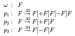An example stochastic L-System where each production rule is applied with a probality of .33.

To add further realism, we also might want to deal with context-sensitive L-systems, rather than the context-free ones we created before. This means that for each application of the production rule, we care about the context of the predecessor string.⁴ For instance, what if a particular branch is pruned off, or has an excess of plant growth hormones, or recieves more nutrients or sunlight.

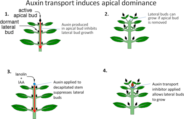Auxins play a role in the coordination of many growth and behavioral processes in plant.

Overall, we’d like to simulate the interaction between plant parts or between neighboring substrings. This particular property makes it such that our L-system is closer to that of a cellular automata which is context-sensitive or where each cell cares about the values in its neighboring cells.

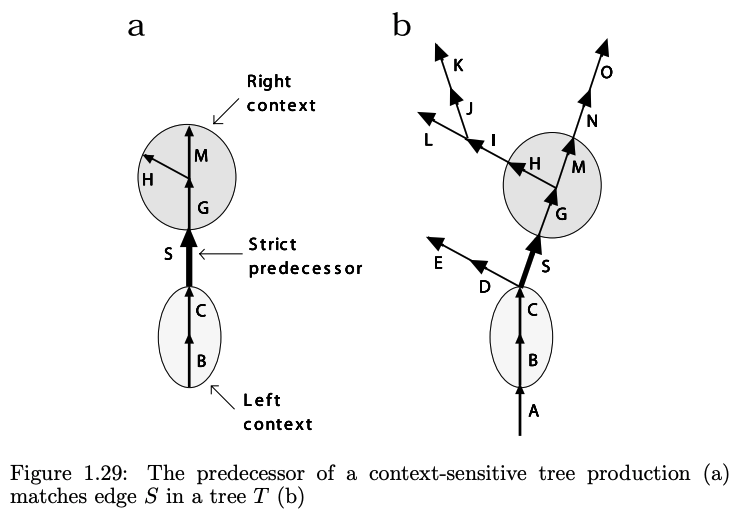An example of a context-sensitive L-System from pg 31 of *The Algorithmic Beauty of Plants*.

This latter context-sensitive property grants us more than one might realize at first glance. Probably the most important biologically relevant phenomenon that it allows us to capture is that of signal propagation (which has found many applications⁷⁸⁹, but imagine implementing an entire neural network, signal propagation and all, in terms of L-systems!)

As an example, let us use this context-sensitivity to simulate signal propagation through a string of symbols,

ω : Baaaaaaaa

p1 : B<a → B

p2 : B → a

If you notice in our first production rule, we have a conditional built into it to check the local surrounding context. This allows us to move the letter B from the left side of a string to the right side through comparisons done between neighboring symbols,

Baaaaaaaa

aBaaaaaaa

aaBaaaaaa

aaaBaaaaa

aaaaBaaaa

···

To extend this topologically 1-dimensional case to that of a more complicated tree structure, we can instead perform comparisons between a path l and an axial tree r and then replacing it with an edge S. This asymmetry between the left context and right context was done because it captures the notion that there is only a single path from the root of a tree to a given edge, but there can be many paths from this edge to different terminal nodes.

This context comparison gets slightly more trickier in the case of bracketed trees. This is because the bracketed string representation does not preserve string neighborhood (rather the brackets are like a memory of past neighborhoods). To solve this we can skip over symbols representing branches or branch portions. The left context in this case would represent signals that propagate outward from the parent root to the children nodes, and the right context would represent signals that propagate inward from the children nodes towards the parent roots.⁴

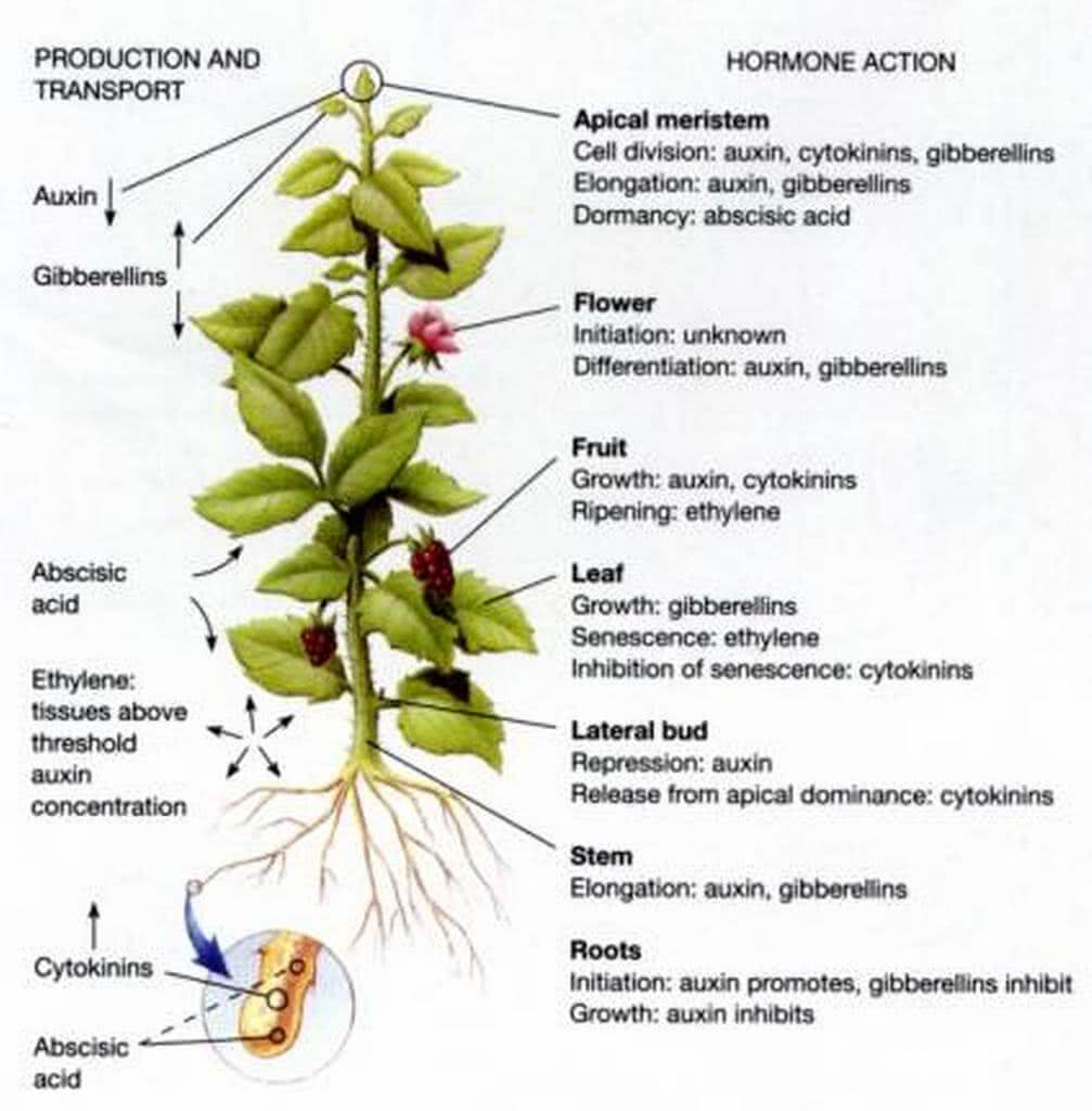Different growth regulating hormones found in plants.

Various other realistic properties can be layered on top of here. Prusinkiewicz and Lindenmayer go on to explain how to implement concepts like exponential growth and other growth functions, diffusion of substances through parametric methods, extending context to overall structure and the external environment through continuous density fields (similar to cellular automata) which allows us to model effects like wind, phototropism and gravity, adding space-time dependent phase effects like that found in different stages of development, adding control mechanisms (like cellular lineage, cell-types, and epigenetic effects), adding cell layers / higher-ordered tissue structure through use of planar graphs with cycles, and more!

I can’t seem to say this enough¹⁰, but really do check out the free copy of The Algorithmic Beauty of Plants when you get a chance, since the authors explain all this in much more depth and beauty than I can at the moment (Professor Prusinkiewicz kindly makes it available for free on his website). In the book they even go on to explain how one should organize their “virtual laboratory” or software environment so as to best experiment and explore these different concepts (pg 193). You can also find various tools and programs that they’ve already written (pg 198).

Breaking down the main plotting code

So now that we understand how the various string compositions that make up our production rules capture different biophysical properties of real-world plants, how do we generate these using Python’s Turtle package?

Following the software philosophy of “Don’t Repeat Yourself” (DRY) we can aim to reduce repetition in coding the above by creating a general purpose program to interpret and generate our strings. This will allow us to reuse the same program and feed it in our different parameters of starting Axiom, Production Rules, Iteration number, Angles, etc, everytime we want to run it with some new combination to generate a different kind of plant structure.

The DRY Principle was formulated by Andy Hunt and Dave Thomas in their book 'The Pragmatic Programmer'. Many widely used programming idioms and phrases were named or popularised by this book such as code katas and rubber duck debugging.

I’ll be breaking down the main plotting code below, but if you want to go straight to experimenting you can go ahead and download the program in my repo here¹¹ and follow the instructions in the README.md on how to input your parameters.

Alternatively, for those that don’t want to do any Python programming, feel free to use an online L-system generator where all you have to do is just input your values (iteration, angle, constants, axiom, and rules) and the plotting will be done instantly within your browser. Nifty!

So getting to our python code, let’s first define some useful functions. We’ll need to create our initial turtle object or pen,

def create_pen(initial_angle):
    '''
    Receives initial orientation / direction given as an draw_angle (ex - 90).
    Returns a turtle object that will be your pen.
    '''
    # Create your pen
    pen = turtle.Turtle() 
    # Specify initial direction you want to draw in
    pen.setheading(initial_angle) 
    # Adjust your pen's width
    pen.pensize(3)
    # Specify a title for your window
    pen.screen.title('L-System')
    # Adjust how fast you want to draw (fastest = 0)
    pen.speed(0)

    return pen

Next, we’ll create a helper function to check if our predecessor string is present. If so, then we’ll replace it with its corresponding successor string,

def production_rule(sequence):
    '''
    Given a predecessor string
    Check if that string is in the dictionary of production rules
    Return the corresponding successor string, 
    Else return what you received
    '''
    # if predecessor string is in the dictionary
    if sequence in DICT_OF_RULES:
        # return the new successor string
        return DICT_OF_RULES[sequence]
    # else if it is not present, just return 
    # the predecessor string mapped to itself
    return sequence

After that, we’ll used that helper function in the next piece of code that applies all of our production rules to our given string,

def apply_production_rules(axiom, iterations):
    '''
    Given an initial string / axiom and amount of iterations
    Apply all the production rules to that list of symbols
    Return a new list of symbols
    '''
    # turn axiom string into a list of substrings
    # in our case, each of these substrings are 
    # an element of our list and each starts out
    # being a single character like F, +, -, etc
    list_of_substrings = [axiom]
    # for each iteration
    for _ in range(iterations):
        # start from the last substring in your list of substrings
        current_substring = list_of_substrings[-1]
        # for each character in that current substring, apply the production rule to it
        new_axiom = [production_rule(char) for char in current_substring]
        # add the new string to the list of substrings
        list_of_substrings.append(''.join(new_axiom))
    return list_of_substrings

Next we’ll need to convert that L-system which is now represented by a long list of states (strings) into its corresponding geometric equivalent. This is the drawing part where we use Turtle,

def draw_L_system(our_pen, DICT_OF_RULES, seg_length, angle):
    # initialize your stack to push and pop your current L-system states 
    stack = []

    # for each symbol in your given string
    for command in DICT_OF_RULES:
        # begin drawing
        our_pen.pendown()

        # R = recursive string-rewriting where symbols on the right side of 
        # the recursive formulas are substituted by corresponding 
        # strings on the left side.  Used to build nodes. 
        # L = recursive string-rewriting where symbols on the left side of 
        # the recursive formulas are substituted by corresponding 
        # strings on the right side.  Used to build nodes. 
        # (see pgs. 15-16 of Algorithmic Botany Textbook)
        if command in ['F', 'R', 'L']:
            # draw one line segment length forward
            our_pen.forward(seg_length)
        elif command == 'f':
            # lift pen up / stop drawing
            our_pen.penup()  
            our_pen.forward(seg_length)
        elif command == "+":
            # turn right
            our_pen.right(angle)
        elif command == "-":
            # turn left
            our_pen.left(angle)
        elif command == "[":
            # push string / state to the memory stack
            stack.append((our_pen.position(), our_pen.heading()))
        elif command == "]":
            # lift pen up / stop drawing
            our_pen.penup()
            # pop string / state off the memory stack
            position, heading = stack.pop()
            our_pen.goto(position)
            our_pen.setheading(heading)

Finally, we’ll need a main function that asks for the various user inputs and uses all the methods above to draw our picture,

def main():

    # Asks user to input their starting Axiom
    axiom = input('Enter starting axiom (w): ')

    # Keep asking user to input their Production rules
    # minimum amount is 1 rule
    production_rule_num = 1 
    while True:
        production_rule = input(f'Enter production rule #{production_rule_num} (Input 0 if no more rules): ')
        
        # Check if there are no more production rules to be entered
        if production_rule == '0':
            break

        # Set key= initial symbol(s) to be replaced  
        # and set value= new symbol(s) you like to replace it with
        key, value = production_rule.split('->')

        # Represents our dictionary of rules
        DICT_OF_RULES[key] = value

        # For aesthetic purposes to help guide the future user input
        production_rule_num += 1

    # Asks user to input their number of iterations to apply their Production Rules   
    iterations = int(input('Enter number of iterations n: '))

    # Asks user to input the desired segment length that is created by Turtle 
    segment_length = int(input('Enter segment length: '))

    # Asks user to input Turtle's initial angle to start drawing towards
    # Angle starts at 3 o'clock and moves in the counterclockwise direction
    initial_angle = float(input('Enter initial angle: '))

    # Asks user to input Turtle's draw_angle to use each time when turning right '+' or left '-'
    draw_angle = float(input('Enter drawing angle: '))

    # Create the whole L-System by applying all the rules the starting axiom
    list_of_entire_L_system = apply_production_rules(axiom, iterations)  # axiom (initial string), nth iterations

    # Initialize Turtle object
    recursive_pen = create_pen(initial_angle)
    # Initialize the background paper or window you'll be drawing on
    window = turtle.Screen()  # create graphics window
    # Set the color of that background
    window.bgcolor('black')
    # Set the size of that background
    window.screensize(1000, 1000)

    # Turn the list representing the entire L-system
    # into an actual geometric drawing
    draw_L_system(recursive_pen, list_of_entire_L_system[-1], segment_length, draw_angle)  # draw list_of_entire_L_system

    # Ensures that the window that you are drawing in 
    # doesn't immediately close after execution
    window.exitonclick()

# Calling main function
if __name__ == "__main__":
    main()

And last but not least, we can run our program on the command line by typing in the following command,

python intro_L_systems.py

And entering the desired inputs,

Enter starting axiom (w): X

Enter production rule 1 (Input 0 if no more rules): X->F-[[X]+X]+F[+FX]-X

Enter production rule 2 (Input 0 if no more rules): F->FF

Enter production rule 3 (Input 0 if no more rules): 0

Enter number of iterations n: 5

Enter segment length: 5

Enter initial angle: 75

Enter drawing angle: 22.5

And our plant is generated! :)

An example of a bracketed L-System representing a type of grass.

Completed image.

Go ahead and play around with inputting other various starting axioms, productions rules, iteration numbers, and angles. Each of the pictures above should give you the required parameters to generate them.

Happy Gardening :) 🌹🌲🌻🌿

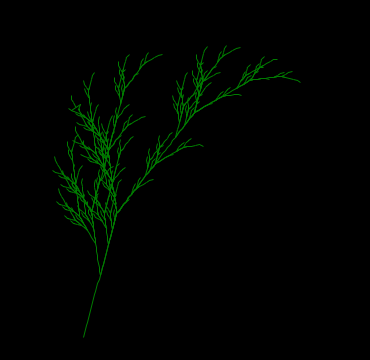
Generating another type of fern.

Moving Forward

In summary, we’ve learned:

• Good practices with Python version management
• How to use the Turtle graphical plotting package
• How to convert between our abstract string rewriting system to a geometric interpretation
• How to implement all this in Python

In the next few articles in this sequence, I’m planning on exploring everything from Cellular Automata, Evolutionary Algorithms, and Neural Networks all from the perspective of Lindenmayer Systems.

Feel free to also check out my book review of The Algorithmic Beauty of Plants on Goodreads!

Resources